Mathematics Class 9 Unit 5: Linear Equations and Inequalities Notes

Linear equations and inequalities are among the most widely used tools in mathematics for modeling real-world relationships and making decisions under constraints. A linear equation in one variable has exactly one solution, found by isolating the variable through balanced operations on both sides. A linear inequality, by contrast, describes a whole range of possible values rather than a single number — its solution set can be represented as an interval on a real line, or, when two variables are involved, as a region of the coordinate plane.

This unit builds from solving simple one-variable equations and inequalities to graphing inequalities in two variables as half planes, and finally to combining several inequalities into a system whose solutions form a feasible region. Every point in that region is a candidate solution to some real-world constraint problem, and the unit closes with the central technique of linear programming: evaluating an objective function at the corner points of the feasible region to find its maximum or minimum value — the same basic idea used in business, engineering, and resource-allocation problems everywhere.

Learning Objectives

• Solve linear equations and inequalities with rational coefficients and represent the solution set on a real line.
• Understand the effect of adding, subtracting, multiplying, and dividing both sides of an inequality, including the sign reversal caused by a negative multiplier or divisor.
• Graph a linear inequality in two variables as a half plane, using a test point to determine the correct shaded region.
• Solve two linear inequalities with two unknowns simultaneously by finding the intersection of their half planes.
• Interpret and identify the feasible region bounded by a system of linear inequalities in two unknowns.
• Identify the corner points (vertices) of a feasible region.
• Find the maximum and minimum values of an objective function by evaluating it at the corner points of the feasible region.

Key Concepts

5.1 Linear Equations in One Variable

A linear equation in one variable has the general form ax + b = 0, where a and b are constants and a ≠ 0, with the highest power of the variable equal to 1. Such an equation always has exactly one solution.

Solving proceeds in four steps: simplify both sides by combining like terms and distributing over parentheses, isolate the variable term by moving all variable terms to one side and constants to the other, solve for the variable by dividing by its coefficient, and finally check the solution by substituting it back into the original equation.

5.2 Linear Inequalities in One and Two Variables

Inequalities use the symbols >, <, ≥, and ≤. Adding or subtracting a constant, or multiplying/dividing by a positive constant, does not change the direction of an inequality — but multiplying or dividing by a negative constant reverses it. A linear inequality in two variables has the form ax + by < c (or >, ≤, ≥), and its associated equation ax + by = c is a line that divides the plane into two half planes.

A vertical line divides the plane into left and right half planes; a non-vertical line divides it into upper and lower half planes. To graph an inequality: draw the associated equation as a dashed line for strict inequalities (< or >) or a solid line for non-strict inequalities (≤ or ≥), then pick a test point not on the line (commonly the origin) to determine which half plane satisfies the inequality.

5.2.2 Systems of Two Linear Inequalities

The graph of a system of linear inequalities is the set of all ordered pairs (x, y) that satisfy every inequality in the system simultaneously. This is found by graphing each inequality's half plane on the same axes and taking their intersection — the overlapping shaded region is the solution region for the whole system.

5.3 Feasible Region and Corner Points

In applied problems, each linear inequality represents a problem constraint, and the full system is the set of problem constraints. Variables are typically restricted to non-negative values (x ≥ 0, y ≥ 0), called non-negative constraints, since they usually represent real quantities like units produced or hours worked. The feasible region is the solution region restricted to the first quadrant, and every point inside it is a feasible solution.

A corner point (or vertex) of the feasible region is a point where two of its boundary lines intersect. Corner points are found either by reading intersection points off the graph or by solving the relevant pairs of boundary equations simultaneously.

5.3.2 Optimizing an Objective Function

A function to be maximized or minimized, subject to the constraints of a feasible region, is called an objective function. Because a feasible region generally contains infinitely many points, the key theorem used in linear programming is that the optimal (maximum or minimum) value of a linear objective function always occurs at one of the corner points of the feasible region — never at an interior point.

The procedure is: graph the constraint inequalities to find the feasible region, identify all corner points, then evaluate the objective function at each corner point and compare the results — the largest value gives the maximum, the smallest gives the minimum.

Important Definitions

Key Facts and Relations

Topic	Key Fact / Relation
ax + b = 0, a ≠ 0	General form of a linear equation in one variable.
ax + by = c	Associated equation of a linear inequality in two variables; a line dividing the plane into two half planes.
If k < 0: a < b ⇒ ka > kb	Multiplying or dividing an inequality by a negative constant reverses its direction.
Test point rule	Substitute the test point into the inequality: if true, its half plane is the solution; if false, the opposite half plane is the solution.
Feasible region = ⋂ (half planes)	The feasible region is the intersection of all half planes defined by the system's constraints, restricted to x ≥ 0, y ≥ 0.
Optimal solution = max/min of f at corner points	The maximum or minimum of the objective function over the feasible region occurs at one of its corner points.

Diagrams

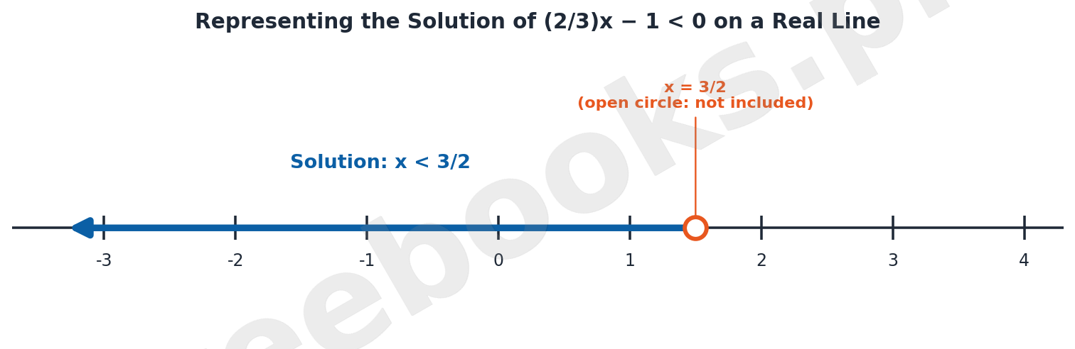
Representing an Inequality's Solution on a Real Line: A number-line diagram showing the open-circle boundary and shaded ray representing the solution x < 3/2 of a linear inequality

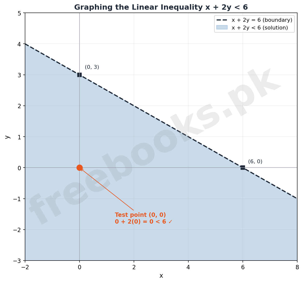
Graphing a Linear Inequality as a Half Plane: A shaded half-plane diagram for x + 2y < 6, showing the dashed boundary line, intercepts, and the origin used as a test point

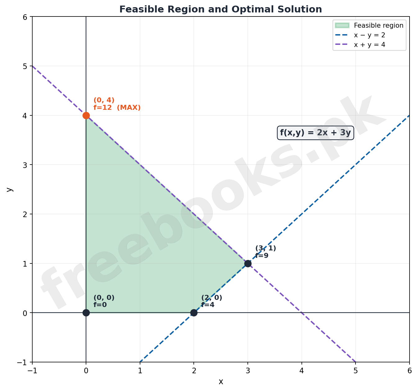
Feasible Region and Optimal Solution: A shaded feasible region bounded by two constraint lines and the axes, with corner points labeled by their objective function values, showing the maximum at (0,4)

Solved Examples

Example 1: Solving a Linear Equation With a Fractional Expression

Problem: Solve (x − 2)/5 − (x − 4)/2 = 2 and check the solution.

1. Combine the fractions over a common denominator of 10: [2(x−2) − 5(x−4)] / 10 = 2.
2. Expand the numerator: 2x − 4 − 5x + 20 = −3x + 16, so (−3x + 16)/10 = 2.
3. Multiply both sides by 10: −3x + 16 = 20.
4. Isolate x: −3x = 4, so x = −4/3.
5. Check by substituting x = −4/3 back into the original equation; both sides simplify to 2, confirming the solution.

Example 2: Solving and Graphing a One-Variable Inequality

Problem: Find the solution of (2/3)x − 1 < 0 and represent it on a real line.

1. Add 1 to both sides: (2/3)x < 1.
2. Multiply both sides by 3 (positive, so direction unchanged): 2x < 3.
3. Divide both sides by 2: x < 3/2.
4. Represent the solution as the open interval (−∞, 3/2) on a real line, with an open circle at 3/2 since it is not included.

Example 3: Graphing a Linear Inequality in Two Variables

Problem: Solve the inequality x + 2y < 6 by graphing its solution region.

1. Write the associated equation x + 2y = 6, which crosses the axes at (6, 0) and (0, 3).
2. Draw this line using dashes, since the inequality is strict (<).
3. Choose the origin (0, 0) as a test point since it is not on the line.
4. Substitute: 0 + 2(0) = 0 < 6, which is true, so the origin's side of the line is the solution region.
5. Shade the half plane containing the origin — the region below the line.

Example 4: Solving a System of Two Linear Inequalities

Problem: Find the solution region for the system x − 2y ≤ 6 and 2x + y ≥ 2.

1. Graph the associated equation x − 2y = 6 using intercepts (6, 0) and (0, −3) as a solid line, since the inequality is non-strict.
2. Test the origin: 0 − 2(0) = 0 < 6, true, so shade the half plane containing the origin.
3. Graph the associated equation 2x + y = 2 using intercepts (1, 0) and (0, 2) as a solid line.
4. Test the origin: 2(0) + 0 = 0, which is not ≥ 2, so shade the half plane not containing the origin.
5. The solution region of the system is the overlap (intersection) of both shaded half planes.

Example 5: Finding the Feasible Region and Its Corner Points

Problem: Shade the feasible region for x − y ≤ 3, x + 2y ≤ 6, x ≥ 0, y ≥ 0, and find its corner points.

1. Graph x − y = 3 as a solid line through (3, 0) and (0, −3); test the origin (0 < 3, true) to shade the origin's side.
2. Graph x + 2y = 6 as a solid line through (6, 0) and (0, 3); test the origin (0 < 6, true) to shade the origin's side.
3. Restrict to the first quadrant by intersecting with x ≥ 0 and y ≥ 0.
4. The resulting feasible region is bounded by the four constraints, with corner points (0, 0), (3, 0), (4, 1), and (0, 3).

Example 6: Finding the Maximum and Minimum of an Objective Function

Problem: Find the maximum and minimum values of f(x, y) = 2x + 3y subject to x − y ≤ 2, x + y ≤ 4, x ≥ 0, y ≥ 0.

1. Graph both constraint lines and restrict to the first quadrant to find the feasible region ABCD.
2. Identify the corner points: (0, 0), (2, 0), (3, 1), and (0, 4).
3. Evaluate f at each corner: f(0,0) = 0, f(2,0) = 4, f(3,1) = 2(3)+3(1) = 9, f(0,4) = 2(0)+3(4) = 12.
4. Compare the values: the minimum is 0 at (0, 0) and the maximum is 12 at (0, 4).

Example 7: Solving an Inequality Involving a Vertical Boundary Line

Problem: Solve the inequality 2x ≥ −3 in the xy-plane.

1. Rewrite as 2x + 0y ≥ −3 to treat it as a two-variable inequality.
2. Solve for x: x ≥ −3/2, so the solution set is all points (x, y) with x, y ∈ ℝ and x ≥ −3/2.
3. The associated equation 2x = −3 is a vertical line parallel to the y-axis.
4. The graph consists of the boundary line and the closed half plane to the right of it.

Example 8: Real-World Application: Maximizing Profit With Linear Programming

Problem: A furniture maker earns profit modeled by f(x, y) = 3x + 5y, where x and y are units of two products, subject to 2x + y ≤ 10, x + 2y ≤ 14, x ≥ 0, y ≥ 0. Find the corner points and the production plan that maximizes profit.

1. Graph 2x + y = 10 with intercepts (5, 0) and (0, 10); test the origin (true) to shade its side.
2. Graph x + 2y = 14 with intercepts (14, 0) and (0, 7); test the origin (true) to shade its side.
3. Restrict to the first quadrant and find the feasible region's corner points: (0, 0), (5, 0), (2, 6), and (0, 7).
4. Evaluate f at each: f(0,0)=0, f(5,0)=15, f(2,6)=6+30=36, f(0,7)=35.
5. The maximum profit of 36 occurs at (2, 6), so the maker should produce 2 units of the first product and 6 of the second.

Short Questions & Answers

Long Questions & Answers

Explain the complete procedure for graphing a system of two linear inequalities in two variables.

What is the first step in graphing an inequality?

Write the associated (corresponding) equation by replacing the inequality symbol with an equal sign, then find its x- and y-intercepts to plot the line.

How is the boundary line drawn?

The line is drawn dashed if the inequality is strict (< or >), or solid if the inequality is non-strict (≤ or ≥), since a solid line indicates the boundary itself is part of the solution.

How is the correct half plane identified?

A test point not on the line — usually the origin — is substituted into the inequality; if it satisfies the inequality, that side is shaded, otherwise the opposite side is shaded.

How is the solution to a system of two inequalities found?

Each inequality's half plane is graphed on the same axes, and the overlapping (intersecting) region of both shaded half planes is the solution region for the whole system.

Describe how the feasible region is used to solve a linear programming problem, with an example.

What is a feasible region and how is it obtained?

A feasible region is the solution region of a system of problem-constraint inequalities restricted to the first quadrant (x ≥ 0, y ≥ 0), found by graphing and intersecting all the constraint half planes.

What is a corner point and why does it matter?

A corner point is a vertex of the feasible region where two boundary lines meet; the maximum or minimum value of a linear objective function is always found at one of these points, not inside the region.

What is the step-by-step procedure to find an optimal solution?

Graph the constraints to determine the feasible region, list all its corner points, then evaluate the objective function at each corner point.

How is the final answer determined from the evaluated values?

The corner point giving the largest value of the objective function is the maximizing solution, and the one giving the smallest value is the minimizing solution — as illustrated by f(x,y)=2x+3y reaching its maximum of 12 at (0,4).

Multiple Choice Questions (MCQs)

Quick Revision Summary

• A linear equation in one variable always has exactly one solution; solve by isolating the variable through balanced operations.
• Multiplying or dividing an inequality by a negative number reverses its direction — this is the single most common source of errors.
• A dashed boundary line means strict inequality (< or >); a solid line means non-strict (≤ or ≥).
• Use a test point, usually the origin, to determine which half plane satisfies an inequality.
• The solution of a system of inequalities is the intersection of all the individual half planes.
• The optimal value of a linear objective function always occurs at a corner point of the feasible region — evaluate the function at every corner point to find it.

Exam Tips

• Always check a solved equation by substituting the answer back into the original equation.
• When multiplying or dividing an inequality by a negative number, flip the inequality symbol immediately — don't wait until the end.
• Pick a test point that is clearly not on the boundary line; the origin works unless the line itself passes through (0,0).
• Sketch all constraint lines on the same axes before shading, so the final feasible region is easy to see.
• List every corner point of the feasible region methodically before evaluating the objective function, so none are missed.
• In word problems, remember that x ≥ 0 and y ≥ 0 constraints restrict the feasible region to the first quadrant only.