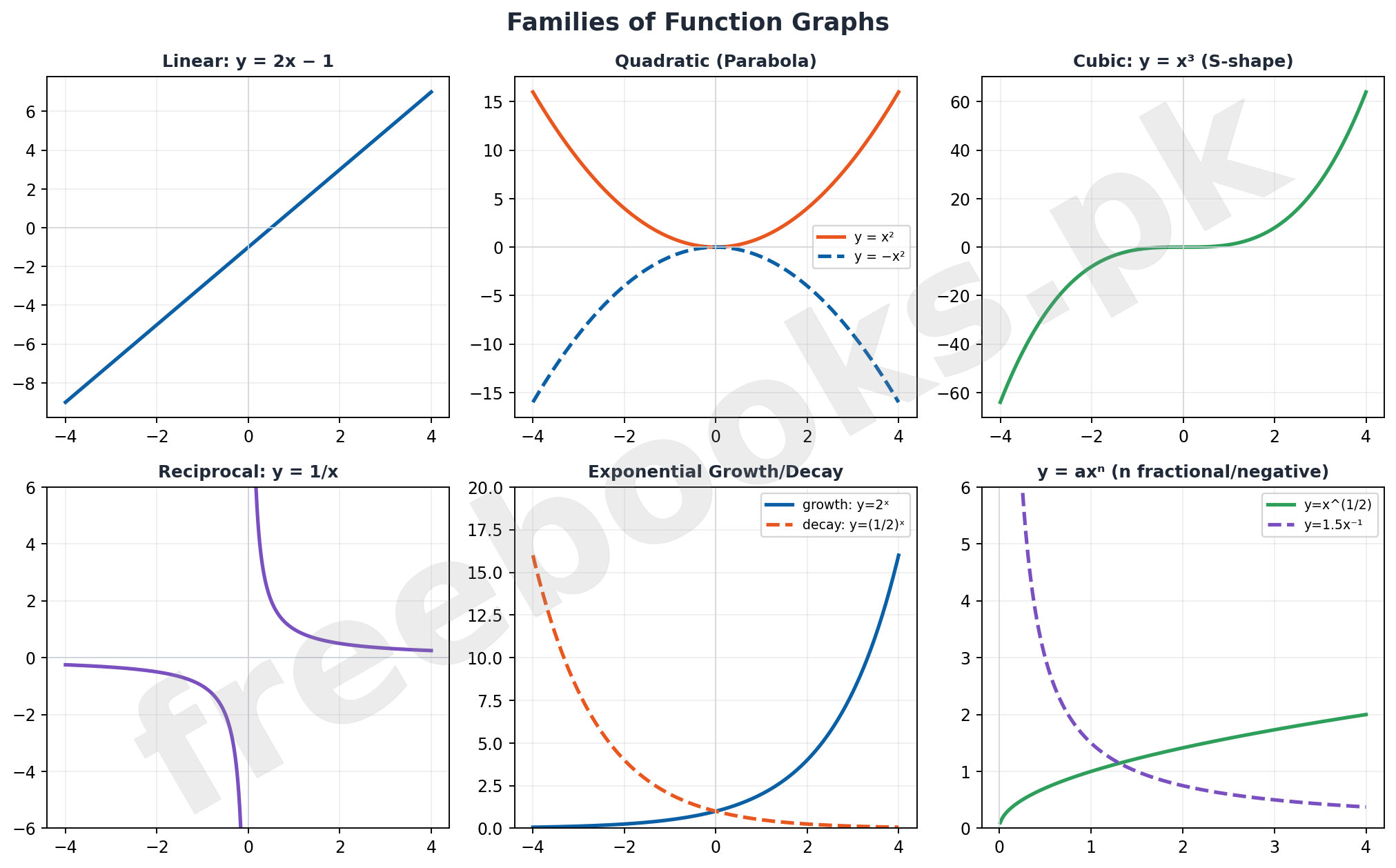
A graph turns an abstract equation into a visual shape, making it far easier to understand how one quantity changes in response to another. This unit builds a visual toolkit for the major function families encountered in school mathematics: linear functions, whose graphs are straight lines; quadratic and cubic functions, whose graphs are curved parabolas and S-shaped curves respectively; reciprocal functions, whose graphs split into separate branches approaching invisible boundary lines called asymptotes; and exponential functions, whose graphs capture the runaway growth or steady decay seen throughout nature and finance.
Beyond simply plotting points, the unit teaches how to read meaning out of a graph — estimating a value at a point that wasn't directly calculated, finding the steepness (gradient) of a curve at a specific point by drawing its tangent line, and recognizing exponential growth or decay from a graph's shape alone. The unit closes with genuinely practical applications: sketching a salary function to see how pay grows with experience, and graphing cost and revenue functions together to find a business's break-even point — the exact production level where profit turns from negative to positive.
Learning Objectives
- Recall and sketch graphs of linear functions of the form y = mx + c.
- Plot and interpret graphs of quadratic functions y = ax² + bx + c, recognizing the parabola shape and its direction of opening.
- Plot and interpret graphs of cubic functions y = ax³ + bx² + cx + d and describe their general S-shaped behavior.
- Plot and interpret graphs of reciprocal functions y = a/x, including their asymptotic behavior.
- Graph y = axⁿ for positive integer, negative integer, and rational values of n (for x > 0).
- Graph exponential functions y = kaˣ (a > 1) and distinguish exponential growth from decay.
- Determine the gradient of a curve at a point by drawing a tangent line and computing its slope.
- Apply graph sketching and interpretation to real-life problems such as salary growth, tax payment, and cost-profit break-even analysis.
Key Concepts
10.1 Functions and Their Graphs
A function y = f(x) expresses a dependent variable y in terms of an independent variable x — f can be represented as an equation, a graph, a table of values, or a verbal description. Graphing a function means plotting the set of all points (x, f(x)) that satisfy the relationship, giving a visual picture of how output changes as input changes.
10.1.1 – 10.1.2 Linear and Quadratic Functions
A linear function f(x) = mx + c graphs as a straight line, with m controlling the steepness (slope) and c giving the y-intercept. Its graph is sketched most easily by finding the x- and y-intercepts (setting y = 0 and x = 0 respectively) and joining them with a straight line.
A quadratic function y = ax² + bx + c (a ≠ 0) always graphs as a parabola: it opens upward if a > 0 and downward if a < 0. The parabola's key features — where it crosses the x-axis and y-axis, and its turning point — are found from a table of values or algebraic analysis.
10.1.3 – 10.1.4 Cubic and Reciprocal Functions
A cubic function y = ax³ + bx² + cx + d (a ≠ 0) graphs as a curve with an S-shaped appearance and at most two turning points; its exact shape varies more than linear or quadratic graphs depending on the coefficients.
A reciprocal function y = a/x (x ≠ 0) produces two separate curve branches — commonly one in each of two opposite quadrants — that approach the x-axis and y-axis (its asymptotes) but never touch them, since the function is undefined at x = 0.
10.1.5 – 10.1.6 Exponential Functions and y = axⁿ
An exponential function y = kaˣ (a > 1) grows increasingly steeply as x increases — this shape represents growth, common in population models, compound interest, and epidemic spread. The constant e ≈ 2.72 gives the especially important natural exponential function y = eˣ.
The general power function y = axⁿ behaves very differently depending on n: for positive integer n (like n=3) the graph passes through the origin and rises; for negative integer n (like n=−1) the graph splits into branches approaching the axes as asymptotes; for rational n (like n=1/5) the graph has a smoother, flatter growth curve for x > 0.
10.2 Exponential Growth/Decay and Gradients of Curves
Exponential growth graphs (e.g., population, compound interest) start slowly and accelerate sharply upward over time; exponential decay graphs (e.g., cooling, depreciation) start high and fall sharply before leveling off. Reading these graphs allows estimation of a quantity at any given time without recomputing the full equation.
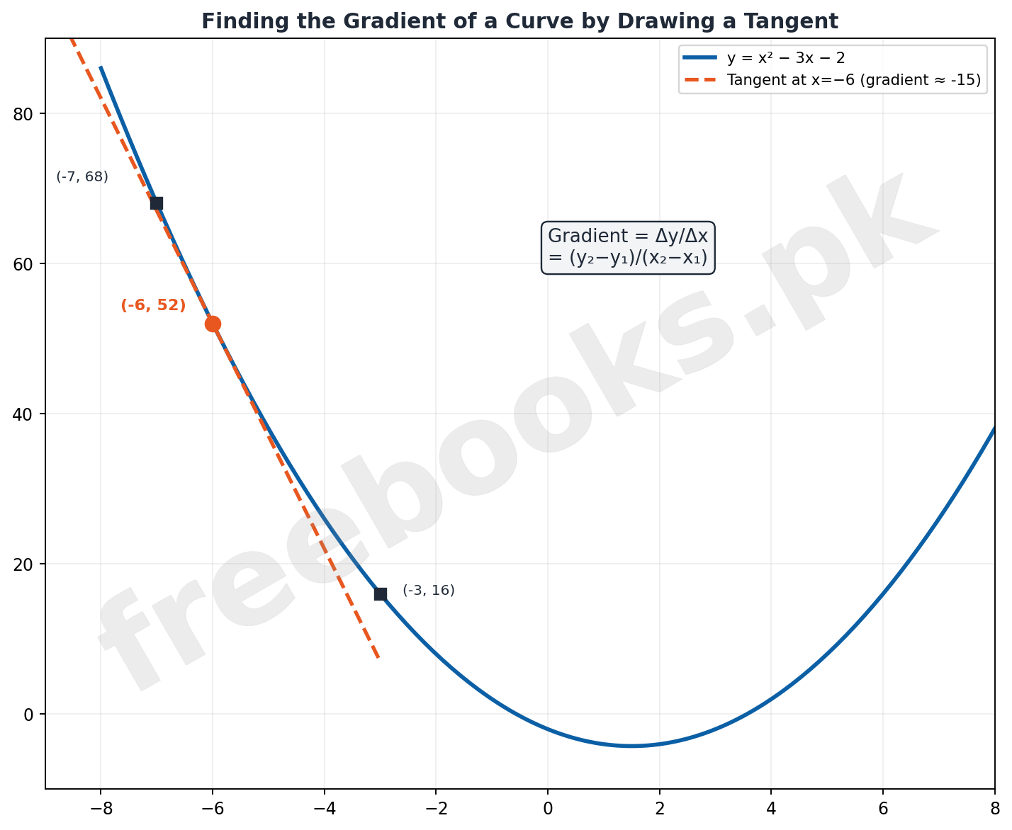
The gradient of a curve at a specific point equals the gradient of the tangent line drawn at that point — a straight line touching the curve at exactly one point without crossing it. Once two points on the tangent line are identified, the gradient is computed the same way as for any straight line: Δy/Δx = (y₂−y₁)/(x₂−x₁).
10.2.2 Real-Life Applications
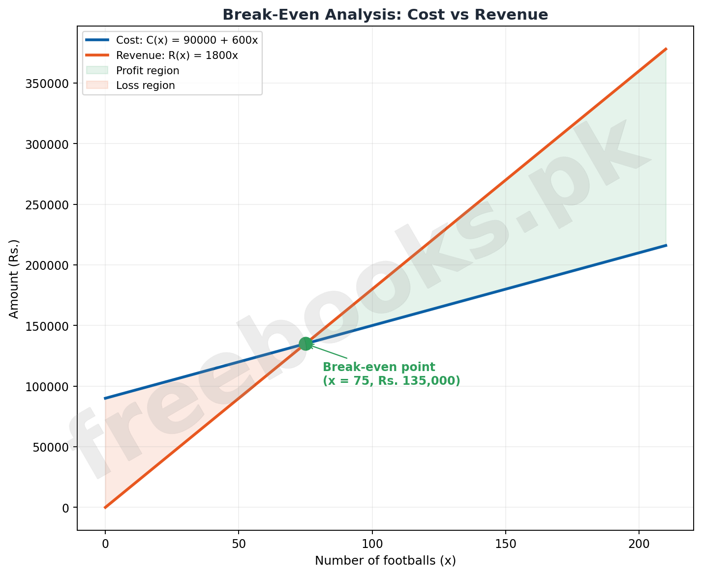
Graphing directly supports practical decision-making: sketching salary versus years of experience reveals the rate of pay growth; graphing tax liability against income can reveal bracket thresholds; and graphing a cost function alongside a revenue function reveals the break-even point — the production level where revenue exactly equals cost, found either graphically (where the two lines intersect) or algebraically (by setting R(x) = C(x) and solving for x).
Important Definitions
Function
A relationship y = f(x) in which each input value x produces exactly one output value y.
Linear Function
A function of the form f(x) = mx + c, whose graph is a straight line with slope m and y-intercept c.
Quadratic Function
A function of the form y = ax² + bx + c (a ≠ 0), whose graph is a parabola opening upward if a > 0 or downward if a < 0.
Cubic Function
A function of the form y = ax³ + bx² + cx + d (a ≠ 0), whose graph is an S-shaped curve with at most two turning points.
Reciprocal Function
A function of the form y = a/x (x ≠ 0), whose graph consists of two separate branches approaching the axes as asymptotes.
Asymptote
A line that a graph approaches ever more closely but never actually touches or crosses.
Exponential Function
A function of the form y = kaˣ (a > 1), whose graph rises with increasing steepness, representing growth.
Tangent Line
A straight line that touches a curve at exactly one point without crossing it there.
Gradient of a Curve at a Point
The slope of the tangent line drawn to the curve at that specific point, computed as Δy/Δx.
Break-Even Point
The production or sales level at which total revenue exactly equals total cost, so profit is zero — found by solving R(x) = C(x).
Key Facts and Relations
| Topic | Key Fact / Relation |
|---|---|
| f(x) = mx + c | General form of a linear function; m is the slope, c is the y-intercept. |
| y = ax² + bx + c, a ≠ 0 | General form of a quadratic function, graphing as a parabola. |
| y = ax³ + bx² + cx + d, a ≠ 0 | General form of a cubic function, graphing as an S-shaped curve. |
| y = a/x, x ≠ 0 | General form of a reciprocal function, with the axes as asymptotes. |
| y = kaˣ, a > 1 | General form of an exponential growth function. |
| y = axⁿ | General power function; behavior depends on whether n is a positive integer, negative integer, or rational number. |
| Gradient = Δy/Δx = (y₂−y₁)/(x₂−x₁) | Formula for the gradient of a line or tangent, using two points on it. |
| Break-even: R(x) = C(x) | Condition defining the break-even point, where revenue equals cost. |
| P(x) = R(x) − C(x) | Profit function, equal to revenue minus cost. |
Diagrams
Families of Function Graphs: A six-panel gallery showing the characteristic shapes of linear, quadratic, cubic, reciprocal, exponential, and power (axⁿ) function graphs
Finding the Gradient of a Curve by Drawing a Tangent: A parabola with a tangent line drawn at a point, showing how two points on the tangent give the gradient via Δy/Δx
Break-Even Analysis: Cost vs Revenue: Cost and revenue lines plotted together, showing their intersection at the break-even point with profit and loss regions shaded
Solved Examples
Example 1: Sketching a Linear Function Using Intercepts
Problem: Sketch the graph of y = 2x − 1.
- Find the y-intercept by setting x = 0: y = 2(0) − 1 = −1, giving the point (0, −1).
- Find the x-intercept by setting y = 0: 0 = 2x − 1, so x = 1/2, giving the point (1/2, 0).
- Plot both intercepts on the coordinate plane and join them with a straight line.
- Since the slope (2) is positive, the line rises from left to right.
Example 2: Sketching a Quadratic Function From a Table of Values
Problem: Sketch the graph of y = 2x² − 7x − 9 for −3 ≤ x ≤ 6.
- Build a table of x and corresponding y values across the given interval by substituting each x into the equation.
- Plot each (x, y) pair as a point on the coordinate plane.
- Connect the points with a smooth curve, since a is positive (a=2), confirming the parabola opens upward.
- Read off where the curve crosses the axes: y-axis at (0, −9), x-axis near (−1, 0) and (4.5, 0).
Example 3: Plotting a Reciprocal Function and Identifying Its Asymptotes
Problem: Sketch the graph of y = 1/(x − 0.5), x ≠ 0.5.
- Build a table of values on either side of the undefined point x = 0.5, using values close to and far from it.
- Note that as x approaches 0.5 from either side, y grows without bound — this identifies x = 0.5 as a vertical asymptote.
- Note that as x becomes very large or very negative, y approaches 0 — this identifies y = 0 as a horizontal asymptote.
- Plot the two separate branches of the curve, each approaching but never touching these asymptotes.
Example 4: Modeling Exponential Population Growth From a Graph
Problem: A village's population follows p = 753e^(0.03t). Graph the population from t=0 to t=30 and estimate the population in 2020 (t=10) and 2030 (t=20).
- Build a table of (t, p) values by substituting t = 0, 5, 10, …, 30 into the equation.
- Plot the points and connect them with a smooth upward curve, characteristic of exponential growth.
- Read the estimated value directly off the graph at t = 10: approximately 1016 persons (year 2020).
- Read the estimated value directly off the graph at t = 20: approximately 1372 persons (year 2030).
Example 5: Finding the Gradient of a Curve by Drawing a Tangent
Problem: Sketch y = x² − 3x − 2 for −8 ≤ x ≤ 8, draw a tangent at x = −6, and determine its gradient.
- Build a table of values and plot the curve across the given interval.
- Draw a straight line that just touches the curve at x = −6 without crossing it — the tangent line.
- Choose two clear points on the tangent line, such as (−3, 10) and (−7, 70).
- Compute the gradient: (70 − 10)/(−7 − (−3)) = 60/(−4) = −15, indicating the curve is decreasing as x increases at this point.
Example 6: Real-World Application: Interpreting a Linear Salary Graph
Problem: Majid's salary is S(x) = 25000 + 1500x, where x is years worked. Sketch and interpret the graph for 0 ≤ x ≤ 10.
- Build a table of values by substituting x = 0, 2, 4, 6, 8, 10 into the salary formula.
- Plot the points; since the formula is linear, they lie on a straight line.
- Observe the y-intercept, 25000, representing the starting salary at x = 0.
- Interpret the slope, 1500, as the fixed salary increase (in rupees) for every additional year worked.
Example 7: Real-World Application: Finding a Break-Even Point Graphically and Algebraically
Problem: A company's cost is C(x) = 90,000 + 600x and revenue is R(x) = 1,800x for producing/selling x footballs. Find the break-even point and the profit at x=150.
- Set revenue equal to cost to find the break-even point algebraically: 1800x = 90000 + 600x.
- Solve: 1200x = 90000, so x = 75 — the break-even point occurs at 75 footballs.
- Compute revenue and cost at x = 150: R(150) = Rs. 270,000, C(150) = Rs. 180,000.
- Compute the profit: P(150) = R(150) − C(150) = Rs. 270,000 − Rs. 180,000 = Rs. 90,000.
Example 8: Comparing Exponential Growth and Decay Shapes
Problem: Plot y = 2ˣ and y = 2⁻ˣ on the same diagram for −4 ≤ x ≤ 4 and describe the difference in their shapes.
- Build a table of values for y = 2ˣ, noting it grows rapidly as x increases and approaches 0 as x decreases.
- Build a table of values for y = 2⁻ˣ = (1/2)ˣ, noting it falls rapidly as x increases and grows large as x decreases.
- Plot both curves on the same axes, observing they are mirror images of each other across the y-axis.
- Conclude that y = 2ˣ represents exponential growth while y = 2⁻ˣ represents exponential decay.
Short Questions & Answers
What information do the x- and y-intercepts give when sketching a linear function?
They provide two points that lie exactly on the line, which is enough to draw the entire straight-line graph.
How does the sign of a in y = ax² + bx + c affect the parabola's shape?
If a > 0 the parabola opens upward; if a < 0 the parabola opens downward.
What is an asymptote?
A line that a graph approaches increasingly closely but never actually touches or crosses.
What distinguishes an exponential growth graph from an exponential decay graph?
A growth graph rises increasingly steeply as x increases, while a decay graph falls sharply and then levels off as x increases.
How is the gradient of a curve at a specific point found?
By drawing the tangent line to the curve at that point, then computing the gradient of that tangent line using two points on it.
What does the y-intercept of a salary function like S(x) = 25000 + 1500x represent?
The starting salary before any years of service have been counted, i.e., the salary at x = 0.
How is the break-even point of a business found algebraically?
By setting the revenue function equal to the cost function, R(x) = C(x), and solving for x.
Long Questions & Answers
Describe the characteristic graph shapes of linear, quadratic, cubic, reciprocal, and exponential functions.
What does a linear function's graph look like?
A straight line, with the slope m controlling its steepness and direction, and the y-intercept c marking where it crosses the y-axis.
What does a quadratic function's graph look like?
A parabola, always symmetric about a vertical line through its turning point, opening upward if the leading coefficient is positive and downward if negative.
What does a cubic function's graph look like?
An S-shaped curve with at most two turning points, showing more varied behavior than linear or quadratic graphs depending on its coefficients.
What do reciprocal and exponential graphs look like?
A reciprocal function's graph splits into two branches approaching the x- and y-axes as asymptotes without touching them; an exponential function's graph rises (or falls, for decay) with continuously changing steepness, never touching the x-axis.
Explain how tangent lines are used to find the gradient of a curve, and how break-even analysis uses two graphed functions together.
Why can't the ordinary two-point slope formula be applied directly to a curve?
A curve's steepness constantly changes from point to point, unlike a straight line, so there is no single overall slope — the gradient must instead be found locally at each specific point of interest.
How does a tangent line solve this problem?
By drawing a straight line that touches the curve at exactly one chosen point without crossing it, the (locally straight) tangent line can be treated as an ordinary line, and its gradient is computed the standard way from any two of its own points.
How is a break-even point identified using two functions?
The cost function C(x) and revenue function R(x) are graphed on the same axes; wherever their curves intersect, revenue exactly equals cost, marking the break-even production level.
How does the graph show profit versus loss regions?
To the left of the break-even point, cost exceeds revenue, indicating a loss region; to the right, revenue exceeds cost, indicating a profit region — visually splitting the graph into two economically meaningful zones.
Multiple Choice Questions (MCQs)
x = 5 represents: (A) x-axis (B) y-axis (C) line parallel to x-axis (D) line parallel to y-axis
Correct answer: (D) line parallel to y-axis. x = 5 is a vertical line at x-coordinate 5, parallel to the y-axis.
The slope of the line y = 5x + 3 is: (A) 3 (B) −3 (C) 5 (D) −5
Correct answer: (C) 5. In y = mx + c form, the coefficient of x, which is 5, is the slope.
The y-intercept of y = −2x − 1 is: (A) −2 (B) 2 (C) −1 (D) 1
Correct answer: (C) −1. Setting x = 0 gives y = −1, the y-intercept.
The graph of y = x³ cuts the x-axis at: (A) x = 0 (B) x = 1 (C) x = −1 (D) x = 2
Correct answer: (A) x = 0. Setting y = 0 gives x³ = 0, so x = 0 is the only root.
The graph of y = 3ˣ represents: (A) growth (B) decay (C) both growth and decay (D) a straight line
Correct answer: (A) growth. Since the base 3 > 1, the graph rises with increasing x, representing exponential growth.
The graph of y = −x² + 5 opens: (A) upward (B) downward (C) left (D) right
Correct answer: (B) downward. The coefficient of x² is negative (−1), so the parabola opens downward.
The graph of y = x² − 9 opens: (A) upward (B) downward (C) left (D) right
Correct answer: (A) upward. The coefficient of x² is positive (1), so the parabola opens upward.
y = 5ˣ is a(n) ______ function. (A) linear (B) quadratic (C) cubic (D) exponential
Correct answer: (D) exponential. A function with a constant base raised to a variable power is exponential.
Which of the following is a reciprocal function? (A) y = 7ˣ (B) y = 2/x (C) y = 2x² (D) y = 5x³
Correct answer: (B) y = 2/x. y = 2/x has the form y = a/x, the defining form of a reciprocal function.
y = −3x³ + 7 is a(n) ______ function. (A) exponential (B) cubic (C) linear (D) reciprocal
Correct answer: (B) cubic. The highest power of x is 3, matching the general cubic form ax³+bx²+cx+d.
Quick Revision Summary
- A linear function's graph is found quickly using its x- and y-intercepts, or its slope and one known point.
- A quadratic function's graph is a parabola opening upward if a>0 and downward if a<0; a cubic function's graph is an S-shaped curve with up to two turning points.
- A reciprocal function's graph has two branches approaching asymptotes (lines it never touches) at the axes.
- An exponential function y = kaˣ (a>1) grows increasingly steeply; its mirror image y = ka⁻ˣ decays, flattening out over time.
- The gradient of a curve at a point is found by drawing its tangent line there and computing that line's slope using two of its own points.
- A break-even point is found by setting a business's revenue function equal to its cost function and solving for the production level x.
Exam Tips
- Always build a table of values before attempting to sketch any nonlinear function — a handful of accurate points prevents guessing the curve's shape.
- For quadratics, check the sign of the leading coefficient first — it immediately tells you whether the parabola opens up or down before any plotting.
- For reciprocal functions, plot values very close to the undefined x-value on both sides — this reveals the asymptote's direction and behavior clearly.
- When drawing a tangent by eye, choose two points on the tangent line itself (not on the curve) that are far apart, for a more accurate gradient calculation.
- In break-even problems, always solve R(x)=C(x) algebraically first, then use the graph as a visual confirmation of the same answer.
- Distinguish carefully between exponential growth (a > 1) and decay (0 < a < 1, or equivalently a negative exponent) — the base or exponent sign is the deciding factor.