Mathematics Class 12 Unit 8: Numerical Solutions of Nonlinear Equations Notes

A nonlinear equation f(x)=0 is one where f cannot be written as ax+b — the variable may appear with powers greater than one or inside trigonometric, exponential, or logarithmic functions. While quadratic, cubic, and quartic equations have algebraic formulas for their roots, no general formula exists for degree five or higher, and even when a formula exists it may be too complicated to use. Numerical methods solve this by iteratively producing closer and closer approximations to a root, starting from the Location of Root Theorem: if f is continuous on [a,b] and f(a) and f(b) have opposite signs, at least one root exists in that interval.

This unit develops four methods that build on this idea: the graphical method (a quick visual estimate), the Bisection Method (repeatedly halving the sign-change interval), the Regula-Falsi Method (using a secant line instead of the midpoint for faster convergence), and the Newton-Raphson Method (using the tangent line at each approximation, converging fastest of all when it works). The unit also introduces the Trapezium Rule for numerically estimating definite integrals that resist exact evaluation, and closes with real-life applications in chemistry, medicine, electronics, and cryptography.

Learning Objectives

• Define a nonlinear equation and state the Location of Root Theorem (LRT)
• Identify intervals of sign change for a continuous function and use them to locate roots
• Approximate a root graphically to one or two decimal places
• Apply the Bisection Method to find a root to a specified accuracy using tolerance |f(c)|<10^(-n)/2
• Apply the Regula-Falsi (False Position) Method using the secant-line formula
• Apply the Newton-Raphson Method using the iterative tangent-line formula x_(n+1)=x_n-f(x_n)/f'(x_n)
• Apply the Trapezium Rule to numerically estimate a definite integral
• Apply numerical root-finding methods to real-life problems in chemistry, medicine, electronics, and cryptography

Key Concepts

8.1 The Location of Root Theorem and Graphical Method

A root (or zero) of y=f(x) is a value of x where f(x)=0 — geometrically, where the graph crosses the x-axis. The Location of Root Theorem (LRT) states: if f is continuous on [a,b] and f(a)f(b)<0 (opposite signs), then at least one real root exists in the open interval (a,b), since a continuous graph cannot jump from below to above the x-axis without crossing it. An interval satisfying this condition is called an interval of sign change.

The graphical method approximates a root by plotting y=f(x) over its interval of sign change and reading off where the curve crosses the x-axis; it gives one or two decimal places of accuracy and is often used to obtain a good starting guess for the more precise numerical methods that follow.

8.2 Accuracy, Tolerance, and the Bisection Method

Before applying a numerical method, a tolerance is set based on the number of decimal places n required: the root c is accepted once |f(c)| < 10^(-n)/2 (e.g. for 2 decimal places, |f(c)|<0.005, rounded to 0.01). All intermediate calculations should be carried out to at least n+1 decimal places, and calculators should be set to radian mode whenever trigonometric functions are involved.

The Bisection Method repeatedly halves the sign-change interval: compute the midpoint c=(a+b)/2, check f(c); if f(a)f(c)<0 the root lies in [a,c] (set b=c), otherwise it lies in [c,b] (set a=c); repeat until |f(c)| is within tolerance. It is simple and guaranteed to converge, but relatively slow since the interval only halves each step.

8.3 Regula-Falsi and Newton-Raphson Methods

The Regula-Falsi (False Position) Method improves on bisection by using the secant line through (a,f(a)) and (b,f(b)) instead of the plain midpoint: c = [af(b)-bf(a)] / [f(b)-f(a)]. Since this weights the estimate toward whichever endpoint is closer to zero, it usually converges faster than bisection, though it still relies only on function values (not derivatives) and the LRT sign-change condition.

The Newton-Raphson Method uses the tangent line to y=f(x) at the current approximation x_n, and takes the tangent's x-intercept as the next approximation: x_(n+1) = x_n – f(x_n)/f'(x_n). It requires f to be differentiable with f'(x)≠0 near the root, and typically converges much faster than bisection or regula-falsi, but does not directly use the LRT and can fail to converge if the initial guess is poor or f'(x_n) is near zero.

8.4 The Trapezium Rule for Numerical Integration

Many definite integrals (like integral of e^(-x^2)) cannot be evaluated by elementary antiderivative methods. The Trapezium Rule approximates integral from a to b of f(x)dx by dividing [a,b] into n equal subintervals of width h=(b-a)/n, treating the area under the curve on each subinterval as a trapezium with parallel sides f(x_(i-1)) and f(x_i), and summing: integral ≈ (h/2)[f(x_0) + 2f(x_1) + 2f(x_2) + … + 2f(x_(n-1)) + f(x_n)].

The approximation improves as n increases, since more (and narrower) trapeziums track the curve's shape more closely; the difference between the trapezium-rule estimate and the exact value (when known via the Fundamental Theorem of Calculus) shrinks toward zero as n grows. The rule works for any continuous function, including those that take negative values, where each trapezium contributes a signed area.

8.5 Real-Life Applications

Numerical root-finding methods solve practical nonlinear equations across many fields: in chemistry, equilibrium concentrations satisfy equations like xe^x=1, solved with Newton-Raphson; in medicine, steady-state heartbeat signal models like x^3-x-1=0 are solved with bisection; in electronics, diode/circuit voltage relationships like sin(V)-0.5V=0 are solved with Regula-Falsi.

In cryptography, key parameters satisfying high-degree polynomial equations (like x^5-10x+5=0) are found using Regula-Falsi or Newton-Raphson to generate secure keys — in every case, the underlying equation resists exact algebraic solution, making systematic numerical iteration the only practical path to an accurate answer.

Important Definitions

Key Facts and Relations

Topic	Key Fact / Relation
Location of Root Theorem condition	f continuous on [a,b] and f(a)f(b) < 0 => at least one root exists in (a,b)
Tolerance for n decimal places	|f(c)| < 10^(-n)/2 (e.g. n=2: |f(c)|<0.005 ≈ 0.01)
Bisection Method	c = (a+b)/2; update a=c or b=c based on sign of f(a)f(c)
Regula-Falsi Method	c = [af(b) – bf(a)] / [f(b) – f(a)]
Newton-Raphson Method	x_(n+1) = x_n – f(x_n)/f'(x_n), requires f'(x_n) ≠ 0
Trapezium Rule	integral(a,b) f(x)dx ≈ (h/2)[f(x_0)+2f(x_1)+…+2f(x_(n-1))+f(x_n)], h=(b-a)/n
Subinterval points for Trapezium Rule	x_i = a + ih, i = 0,1,2,…,n
Single trapezium area	A_i = (h/2)[f(x_(i-1)) + f(x_i)]
Newton-Raphson tangent line	y – f(x_n) = f'(x_n)(x – x_n)
Regula-Falsi secant line	y – f(a) = [f(b)-f(a)]/(b-a) * (x-a)

Diagrams

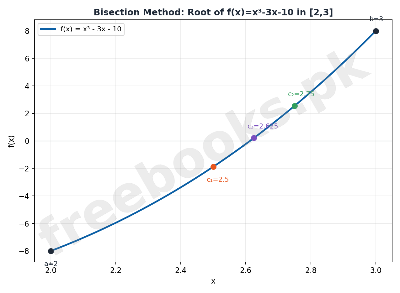
Bisection Method: Repeated Interval Halving: The cubic f(x)=x³-3x-10 on [2,3] with the successive midpoints c₁=2.5, c₂=2.75, c₃=2.625 marked, showing how the Bisection Method narrows in on the root near x≈2.61

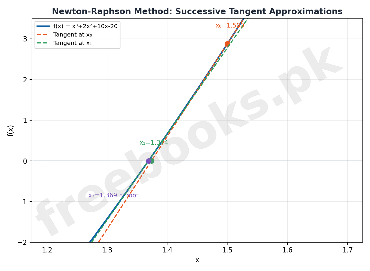
Newton-Raphson Method: Successive Tangent Approximations: The tangent lines drawn at x₀=1.500 and x₁=1.374 for f(x)=x³+2x²+10x-20, showing how each tangent's x-intercept gives a rapidly improving approximation converging to the root near x≈1.37

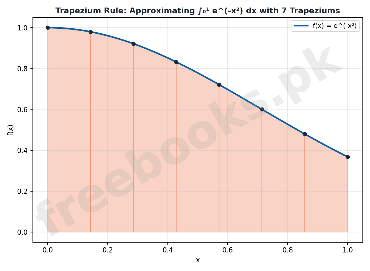
Trapezium Rule: Approximating a Definite Integral: The curve f(x)=e^(-x²) on [0,1] divided into 7 trapeziums, illustrating how the sum of trapezium areas approximates the exact area under the curve

Solved Examples

Example 1: Finding an Interval of Sign Change

Problem: Show that f(x)=x⁴-200x-50 has at least two real roots by finding its intervals of sign change.

1. Confirm f is continuous everywhere, since it is a polynomial: lim as x→c of f(x) = f(c) for all real c.
2. Evaluate f at several integer points: f(-1)=151>0, f(0)=-50<0, f(5)=-425<0, f(6)=46>0.
3. Check the sign of f(-1)·f(0): 151×(-50)<0, so [-1,0] is an interval of sign change.
4. Check the sign of f(5)·f(6): (-425)(46)<0, so [5,6] is another interval of sign change.
5. Final answer: since f is continuous and changes sign on both [-1,0] and [5,6], by the LRT it has at least two real roots.

Example 2: Graphical Method for a Root

Problem: Find a root of x-cos(x)=0 graphically, correct to two decimal places.

1. Define f(x)=x-cos(x) and confirm continuity everywhere (it's a sum of continuous functions).
2. Find an interval of sign change: f(0)=0-cos(0)=-1<0 and f(1)=1-cos(1)≈0.46>0, so [0,1] is an interval of sign change.
3. Compute several function values inside [0,1] (in radian mode) and plot y=x-cos(x) over this interval.
4. Observe where the plotted curve crosses the x-axis.
5. Final answer: the curve crosses the x-axis at approximately x≈0.74.

Example 3: Bisection Method

Problem: Use the Bisection Method to find a root of f(x)=x³-3x-10 in [2,3], accurate to two decimal places.

1. Confirm f(2)=-8<0 and f(3)=8>0, so [2,3] is an interval of sign change, and f (a polynomial) is continuous there.
2. Iteration 1: c=(2+3)/2=2.5, f(2.5)=-1.875<0, so the root lies in [2.5,3].
3. Iteration 2: c=(2.5+3)/2=2.75, f(2.75)≈2.547>0, so the root lies in [2.5,2.75]. Continuing this halving process through further iterations narrows the interval further.
4. After 8 iterations, c≈2.6133 with f(2.6133)≈0.0072, satisfying the tolerance |f(c)|<0.01 for 2 decimal places.
5. Final answer: x ≈ 2.61.

Example 4: Regula-Falsi Method

Problem: Use the Regula-Falsi Method to find a root of f(x)=x³-3x-10 in [2,3], accurate to two decimal places.

1. Confirm f(2)=-8<0 and f(3)=8>0, so a root lies in [2,3].
2. Iteration 1: c = [2(8)-3(-8)]/[8-(-8)] = 40/16 = 2.5; f(2.5)=-1.875<0, so the root lies in [2.5,3].
3. Iteration 2: c = [2.5(8)-3(-1.875)]/[8-(-1.875)] ≈ 2.5949; f(2.5949)≈-0.3119<0, so the root lies in [2.5949,3].
4. Continuing this process, iteration 3 gives c≈2.6101 with f≈-0.0487, and iteration 4 gives c≈2.6125 with f≈-0.0068.
5. Final answer: since |f(2.6125)|≈0.0068<0.01, the root is x ≈ 2.61 (matching the Bisection Method result, but reached in fewer iterations).

Example 5: Newton-Raphson Method

Problem: Use the Newton-Raphson Method to find a root of f(x)=x³+2x²+10x-20, correct to two decimal places.

1. Confirm f(1)=-7<0 and f(2)=16>0, so a root lies in [1,2]; choose initial guess x₀=1.500.
2. Find the derivative: f'(x)=3x²+4x+10, which is never zero (always positive), so the method applies.
3. Iteration 1: f(1.5)=2.875, f'(1.5)=22.750, so x₁ = 1.500 – 2.875/22.750 ≈ 1.374.
4. Iteration 2: f(1.374)≈0.110, f'(1.374)≈21.160, so x₂ = 1.374 – 0.110/21.160 ≈ 1.369.
5. Final answer: f(1.369)≈0.002<0.01, satisfying the tolerance, so x ≈ 1.37.

Example 6: Trapezium Rule for a Definite Integral

Problem: Use the Trapezium Rule to approximate integral from 0 to 1 of e^(-x²)dx, dividing [0,1] into 7 equal subintervals.

1. Compute the step size: h = (1-0)/7 = 1/7 ≈ 0.1429.
2. Compute function values at each x_i (rounded to 4 decimal places): f(0)=1, f(1/7)=0.9798, f(2/7)=0.9216, f(3/7)=0.8322, f(4/7)=0.7214, f(5/7)=0.6004, f(6/7)=0.4797, f(1)=0.3679.
3. Apply the Trapezium Rule: integral ≈ (h/2)[f(x_0) + 2(f(x_1)+…+f(x_6)) + f(x_7)].
4. Substitute: (1/14)[1 + 2(0.9798+0.9216+0.8322+0.7214+0.6004+0.4797) + 0.3679] = (1/14)[1 + 2(4.5351) + 0.3679].
5. Final answer: integral from 0 to 1 of e^(-x²)dx ≈ 0.7456.

Example 7: Real-Life Application: Chemical Equilibrium Concentration

Problem: In a chemical reaction, the equilibrium concentration x (mol/L) satisfies xe^x=1. Find x correct to two decimal places using the Newton-Raphson Method.

1. Define f(x)=xe^x-1 and its derivative f'(x)=e^x+xe^x, which exist for all real x.
2. Check f(0)=-1<0 and f(1)≈1.718>0, so a root lies in [0,1]; since f(0.5)≈-0.1756 is close to zero, take x₀=0.5.
3. Iteration 1: f(0.5)≈-0.1757, f'(0.5)≈2.4730, so x₁ = 0.5 – (-0.1757)/2.4730 ≈ 0.5711.
4. Iteration 2: f(0.5711)≈0.0107, f'(0.5711)≈2.7813, so x₂ = 0.5711 – 0.0107/2.7813 ≈ 0.5673.
5. Final answer: f(0.5673)≈0.0004≈0, so the equilibrium concentration is x ≈ 0.57 moles per liter.

Example 8: Real-Life Application: Electronic Circuit Voltage

Problem: In a circuit, the voltage V satisfies sin(V)-0.5V=0. Find a non-zero value of V correct to two decimal places using the Regula-Falsi Method.

1. Define f(V)=sin(V)-0.5V. Check f(1)=sin(1)-0.5≈0.3415>0 and f(2)=sin(2)-1≈-0.0907<0, so [1,2] is an interval of sign change.
2. Iteration 1: apply the Regula-Falsi formula to get V_c≈1.7901; f(1.7901)≈0.0810>0, so the root lies in [1.7901,2].
3. Iteration 2: V_c≈1.8891; f(1.8891)≈0.0052>0, so the root lies in [1.8891,2].
4. Iteration 3: V_c≈1.8951; f(1.8951)≈0.0003, very close to zero.
5. Final answer: since |f(1.8951)|<0.01, V ≈ 1.90 volts.

Short Questions & Answers

Long Questions & Answers

Compare the Bisection Method, Regula-Falsi Method, and Newton-Raphson Method, explaining how each computes its next approximation and their relative strengths.

How does the Bisection Method compute its next approximation?

It always takes the exact midpoint c=(a+b)/2 of the current sign-change interval, checks which half still contains a sign change, and discards the other half — guaranteed to converge, but relatively slow since it ignores how close each endpoint's function value is to zero.

How does the Regula-Falsi Method improve on this?

Instead of the plain midpoint, it uses the x-intercept of the secant line joining (a,f(a)) and (b,f(b)): c=[af(b)-bf(a)]/[f(b)-f(a)], which is pulled toward whichever endpoint has the smaller |f| value, typically converging faster than bisection while still only needing function values, not derivatives.

How does the Newton-Raphson Method differ from both?

It uses the tangent line to the curve at the current approximation x_n rather than any interval endpoints, taking the tangent's x-intercept x_(n+1)=x_n-f(x_n)/f'(x_n) as the next guess; this typically converges fastest of the three when it works, but requires f to be differentiable with f'≠0 near the root, and does not rely directly on the Location of Root Theorem.

When might Newton-Raphson be a poor choice compared to the other two?

If f'(x_n) is very small or zero near the current approximation, the tangent line becomes nearly horizontal and the next approximation can shoot far away from the root, potentially failing to converge — Bisection and Regula-Falsi, by staying within a guaranteed sign-change interval, avoid this risk entirely.

Explain how the Trapezium Rule is derived and applied, and how its accuracy can be assessed.

How is the interval [a,b] prepared for the Trapezium Rule?

It is divided into n equal subintervals of width h=(b-a)/n, with division points x_i=a+ih for i=0,1,…,n, so each subinterval [x_(i-1),x_i] has the same width h.

How is the area under the curve approximated on each subinterval?

Each subinterval is treated as a trapezium with parallel sides of length f(x_(i-1)) and f(x_i) and height (base) h, giving area A_i=(h/2)[f(x_(i-1))+f(x_i)]; summing all n trapezium areas and combining repeated terms gives the full formula (h/2)[f(x_0)+2f(x_1)+…+2f(x_(n-1))+f(x_n)].

How is the accuracy of a Trapezium Rule estimate checked?

When the exact value of the integral can be found using the Fundamental Theorem of Calculus, the two values are compared directly; the absolute difference gives the error of the approximation, and this error shrinks as n (the number of subintervals) increases.

Does the Trapezium Rule require f(x) to be positive?

No — although it is motivated by approximating area under a positive curve, it is generally valid for any continuous function including one that takes negative values, where each trapezium then represents a signed area contributing to the total integral.

Multiple Choice Questions (MCQs)

Quick Revision Summary

• Nonlinear equation: f(x)=0 where f is not of the form ax+b; root/zero is where the graph crosses the x-axis
• Location of Root Theorem (LRT): f continuous on [a,b], f(a)f(b)<0 => at least one root in (a,b)
• Graphical method: plot f over the sign-change interval, read off where it crosses the x-axis (1-2 decimal places)
• Tolerance for n decimal places: |f(c)| < 10^(-n)/2
• Bisection Method: c=(a+b)/2, halve the interval each iteration based on sign of f(a)f(c)
• Regula-Falsi Method: c=[af(b)-bf(a)]/[f(b)-f(a)], the secant-line x-intercept, converges faster than bisection
• Newton-Raphson Method: x_(n+1)=x_n-f(x_n)/f'(x_n), tangent-line x-intercept, fastest convergence but needs f'≠0
• Trapezium Rule: integral(a,b) f(x)dx ≈ (h/2)[f(x_0)+2f(x_1)+…+2f(x_(n-1))+f(x_n)], h=(b-a)/n
• Trapezium Rule accuracy improves as n increases; works for functions taking negative values too
• Applications: chemical equilibrium (Newton-Raphson), heartbeat models (Bisection), circuit voltages (Regula-Falsi), cryptographic key parameters (Regula-Falsi/Newton-Raphson)

Exam Tips

• Always verify continuity and check f(a)f(b)<0 before applying any LRT-based method (Bisection, Regula-Falsi) — skipping this check can lead to applying the method where no root is guaranteed
• Keep at least one extra decimal place in every intermediate calculation beyond the accuracy you need in the final answer, to avoid compounding rounding errors across iterations
• For Newton-Raphson, always compute f'(x) symbolically once at the start, then substitute numerical values at each iteration — recomputing the derivative formula each time wastes effort and invites errors
• Build an iteration table (columns: iteration, a, b, c, f(c), new interval) for Bisection and Regula-Falsi problems — it keeps the halving/narrowing process organized and easy to check
• Remember trigonometric functions must be evaluated in radian mode throughout every numerical method calculation
• For the Trapezium Rule, always double-check the coefficient pattern (1, 2, 2, 2, …, 2, 1) before summing — forgetting to double the interior terms is the most common calculation error