Mathematics Class 12 Unit 2: Further Differentiation Notes

This unit extends differentiation beyond polynomials and rational functions to trigonometric, inverse trigonometric, exponential, and logarithmic functions, and introduces the chain rule for composite, parametric, and implicit relations. Together these rules make it possible to differentiate almost any function encountered in calculus.

The unit then applies differentiation to real problems: finding equations of tangent and normal lines, computing higher-order derivatives, determining where a function is increasing or decreasing, locating local and global extrema (using critical points and the second derivative test), approximating function values with linearization and differentials (including relative/percentage error), and solving real-world optimization problems by finding the extrema of a modeling function.

Learning Objectives

• Differentiate trigonometric and inverse trigonometric functions, and apply the chain rule to composite, parametric, and implicit relations
• Differentiate exponential and logarithmic functions, including composite forms
• Find equations of tangent and normal lines to a curve at a given point
• Find higher-order derivatives of algebraic, implicit, parametric, and transcendental functions
• Determine intervals where a function is increasing or decreasing using critical points and the sign of the first derivative
• Find local and global extrema of a function using the second derivative test and by checking endpoints
• Use linearization and differentials to approximate function values and compute relative/percentage error
• Apply extrema to solve real-world optimization problems

Key Concepts

2.1 Derivatives of Trigonometric and Inverse Trigonometric Functions, and the Chain Rule

From the limit definition, d/dx(sin x)=cos x and d/dx(cos x)=-sin x; the remaining trig derivatives (tan, cot, sec, csc) follow using the quotient rule, e.g. d/dx(tan x)=sec^2 x. If f(u) is differentiable at u=g(x) and g is differentiable at x, the chain rule gives (f o g)'(x)=f'(g(x)).g'(x), or in Leibniz notation dy/dx=(dy/du)(du/dx) — this same idea extends to parametric equations (dy/dx=(dy/dt)/(dx/dt)) and implicit differentiation (differentiate both sides of F(x,y)=0 with respect to x, applying the chain rule to every y-term, then solve for dy/dx).

The derivatives of the six inverse trigonometric functions are proved by writing y=f^-1(x) as x=f(y), differentiating implicitly, and simplifying using the appropriate Pythagorean identity: d/dx(sin^-1 x)=1/sqrt(1-x^2), d/dx(cos^-1 x)=-1/sqrt(1-x^2), d/dx(tan^-1 x)=1/(1+x^2), d/dx(cot^-1 x)=-1/(1+x^2), d/dx(sec^-1 x)=1/(|x|sqrt(x^2-1)), and d/dx(csc^-1 x)=-1/(|x|sqrt(x^2-1)).

2.2 Derivatives of Exponential and Logarithmic Functions

Using the limit definition and the standard limit lim(h->0)(a^h-1)/h=ln a, the derivative of the exponential function is d/dx(a^x)=a^x ln a, which reduces to d/dx(e^x)=e^x since ln e=1. Composite exponential functions are differentiated with the chain rule: d/dx(a^u)=a^u ln a . du/dx.

Similarly, using the limit definition and lim(h->0)(1+h/a)^(a/h)=e, the derivative of the logarithmic function is d/dx(log_a x)=1/(x ln a), which reduces to d/dx(ln x)=1/x. Composite logarithmic functions follow the same chain rule pattern: d/dx(log_a u)=(1/(u ln a)) du/dx.

2.3 Tangent/Normal Lines and Higher-Order Derivatives

The tangent line to y=f(x) at (x0,f(x0)) is y-y0=m(x-x0) where m=f'(x0); the normal line is perpendicular to the tangent, given by y-y0=-(1/m)(x-x0) when m<>0, or x=x0 when m=0 (and x=x0 is a vertical tangent when m is undefined/infinite).

Since the derivative f' is itself a function, it can be differentiated again to give the second derivative f'', and repeatedly to give third, fourth, and higher-order derivatives, written y', y'', y''', y^(n) or dy/dx, d^2y/dx^2, …, d^n y/dx^n — these are found by simply differentiating the previous derivative again, and can be computed for algebraic, implicit, parametric, and transcendental functions alike.

2.4 Increasing/Decreasing Functions and Extrema

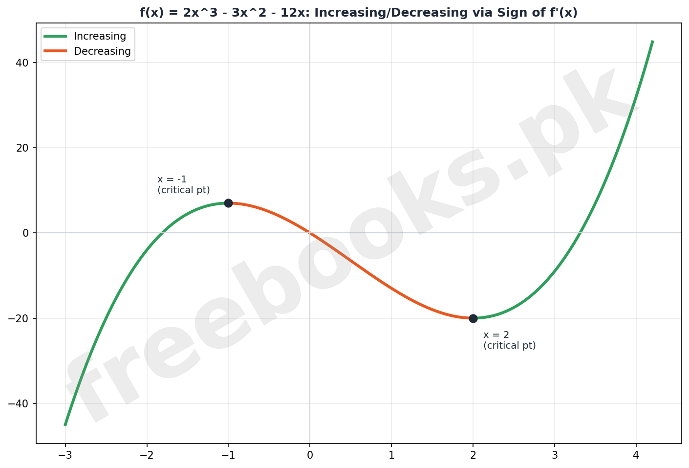
A differentiable function f is increasing on an interval I if f'(x)>=0 throughout I, and decreasing if f'(x)<=0 throughout I. A critical point is a point x=c in the domain where f'(c)=0 (a stationary point) or f'(c) does not exist; critical points divide the domain into subintervals on which the sign of f' stays constant, and testing one point per subinterval determines whether f is increasing or decreasing there.

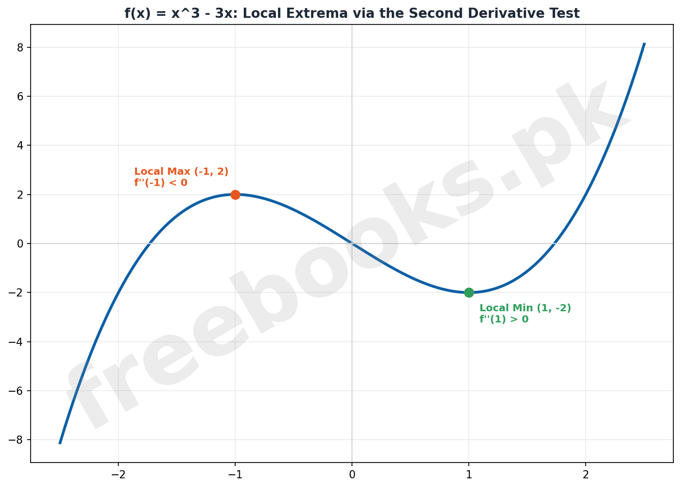
A function has a global (absolute) maximum/minimum at x=c if f(c) is the largest/smallest value on the whole domain, and a local (relative) maximum/minimum if f(c) is the largest/smallest value only in some neighborhood of c. Global extrema on a closed interval [a,b] are found by comparing f at all critical points and at both endpoints; local extrema are classified using the second derivative test: if f'(c)=0, then f has a local max at c if f''(c)<0, a local min if f''(c)>0, and the test is inconclusive if f''(c)=0.

2.5 Linear Approximation and Differentials

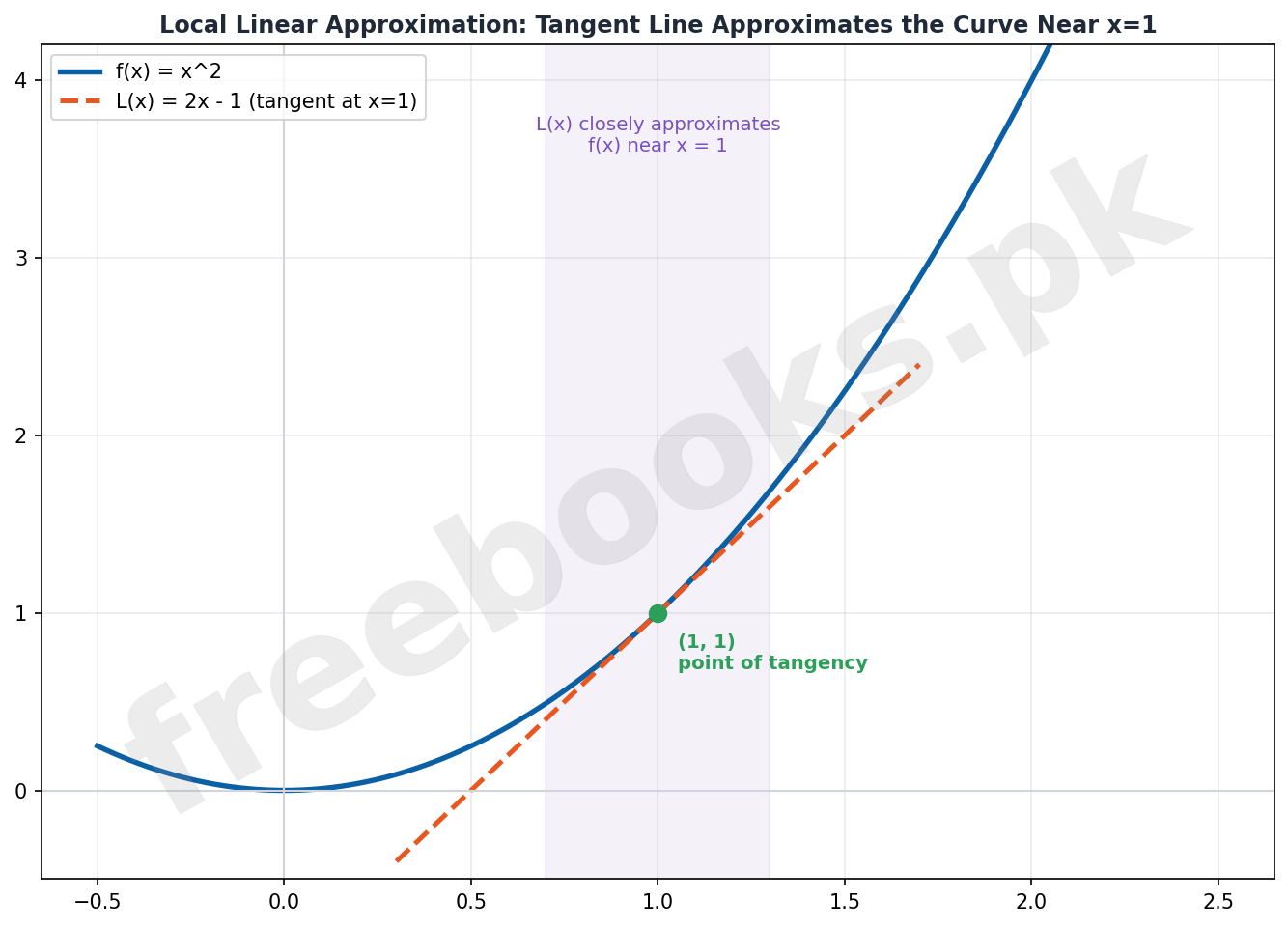
Since a differentiable curve behaves locally like its tangent line, the linearization of f at x=a is L(x)=f(a)+f'(a)(x-a), and f(x) is approximated by L(x) for x near a — useful for quickly estimating values like square roots or trigonometric values near a known point.

For a differentiable function with independent differential dx, the differential dy is defined by dy=f'(x)dx; for small Deltax=dx, the actual change Deltay=f(x+Deltax)-f(x) is approximately equal to dy, so f(x+Deltax) is approximately f(x)+dy. The error in this approximation is Deltay-dy, the relative error is (Deltay-dy)/Deltay, and the percentage error is |((Deltay-dy)/Deltay)|x100 — this same framework estimates the error propagated into a computed quantity (like volume or area) from a small measurement error in a linear dimension.

2.6 Applying Extrema to Real-World Optimization Problems

Optimization problems are solved by: understanding what is to be optimized, assigning variables to the unknowns, writing a function for the quantity to be optimized (using any given constraint to eliminate a variable), finding critical points by differentiating and setting the derivative to zero, confirming maximum or minimum using the second derivative test, and finally interpreting the mathematical answer back in the real-world context.

This method applies broadly — maximizing the area of a fenced garden or an inscribed rectangle, minimizing the material (surface area) of a container of fixed volume, minimizing distance (e.g. signal strength problems), and minimizing algorithm runtime or other modeled quantities — always by reducing the problem to finding the extremum of a single-variable function.

Important Definitions

Key Facts and Relations

Topic	Key Fact / Relation
Derivatives of trig functions	d/dx(sin x)=cos x, d/dx(cos x)=-sin x, d/dx(tan x)=sec^2 x, d/dx(cot x)=-csc^2 x, d/dx(sec x)=sec x tan x, d/dx(csc x)=-csc x cot x
Derivatives of inverse trig functions	d/dx(sin^-1 x)=1/sqrt(1-x^2), d/dx(tan^-1 x)=1/(1+x^2), d/dx(sec^-1 x)=1/(|x| sqrt(x^2-1))
Chain rule	dy/dx = dy/du . du/dx (composite); dy/dx = (dy/dt)/(dx/dt) (parametric)
Exponential and logarithmic derivatives	d/dx(a^x) = a^x ln a; d/dx(log_a x) = 1/(x ln a); d/dx(e^x)=e^x; d/dx(ln x)=1/x
Tangent and normal lines	Tangent: y-y0 = m(x-x0), m=f'(x0); Normal: y-y0 = -(1/m)(x-x0), m<>0
Second derivative test	f'(c)=0: local max if f''(c)<0; local min if f''(c)>0; inconclusive if f''(c)=0
Linearization	L(x) = f(a) + f'(a)(x-a); f(x) is approximately L(x) for x near a
Differential and error	dy = f'(x)dx; Deltay is approximately dy; Percentage Error = |(Deltay-dy)/Deltay| x 100
Global extrema on [a,b]	Compare f at all critical points in [a,b] and at both endpoints x=a, x=b
Optimization method	Define variables -> write function to optimize -> find critical points -> confirm with 2nd derivative test -> interpret result

Diagrams

Increasing/Decreasing via Sign of f'(x): The graph of f(x)=2x^3-3x^2-12x, colored green where increasing and orange where decreasing, with critical points marked at x=-1 and x=2

Local Extrema via the Second Derivative Test: The graph of f(x)=x^3-3x showing a local maximum at (-1,2) where f''<0 and a local minimum at (1,-2) where f''>0

Local Linear Approximation: Tangent Line Near a Point: The graph of f(x)=x^2 together with its tangent line L(x)=2x-1 at x=1, showing that the tangent closely approximates the curve near the point of tangency

Solved Examples

Example 1: Differentiating a Composite Function Using the Chain Rule

Problem: Differentiate y = sin(x^2 – x) with respect to x.

1. Let u = x^2 – x, so that y = sin u.
2. Differentiate y with respect to u: dy/du = cos u.
3. Differentiate u with respect to x: du/dx = 2x – 1.
4. Apply the chain rule: dy/dx = (dy/du)(du/dx) = cos u . (2x-1).
5. Substitute u = x^2-x back: dy/dx = cos(x^2-x)(2x-1).

Example 2: Implicit Differentiation

Problem: Find dy/dx if x + y^2 + sin(xy^2) = 0.

1. Differentiate every term with respect to x, treating y as a function of x: d/dx(x) + d/dx(y^2) + d/dx(sin(xy^2)) = 0.
2. This gives: 1 + 2y(dy/dx) + cos(xy^2) . d/dx(xy^2) = 0.
3. Expand d/dx(xy^2) using the product rule: d/dx(xy^2) = y^2 + x(2y dy/dx), so the equation becomes 1 + 2y(dy/dx) + cos(xy^2){y^2 + 2xy(dy/dx)} = 0.
4. Collect all dy/dx terms on one side: 2y(dy/dx){1 + x cos(xy^2)} = -1 – y^2 cos(xy^2).
5. Solve for dy/dx: dy/dx = -[1 + y^2 cos(xy^2)] / [2y{1 + x cos(xy^2)}].

Example 3: Differentiating a Composite Exponential Function

Problem: Find dy/dx if y = e^(sin^2 x).

1. Apply the chain rule for exponentials: dy/dx = e^(sin^2 x) . d/dx(sin^2 x), since d/dx(e^u)=e^u . du/dx.
2. Differentiate sin^2 x using the chain rule again: d/dx(sin^2 x) = 2 sin x . d/dx(sin x) = 2 sin x cos x.
3. Substitute back: dy/dx = e^(sin^2 x) . 2 sin x cos x.
4. Final answer: dy/dx = 2 sin x cos x . e^(sin^2 x).

Example 4: Finding Higher-Order Derivatives

Problem: Find all higher-order derivatives of y = e^(ax).

1. Differentiate once using the chain rule: dy/dx = e^(ax) . a = a e^(ax).
2. Differentiate again: d^2y/dx^2 = a(a e^(ax)) = a^2 e^(ax).
3. Differentiate a third time: d^3y/dx^3 = a^2(a e^(ax)) = a^3 e^(ax).
4. The pattern continues: d^4y/dx^4 = a^4 e^(ax), and in general d^n y/dx^n = a^n e^(ax) for n>=1.
5. Final answer: d^n y/dx^n = a^n e^(ax) = a^n y.

Example 5: Equations of the Tangent and Normal Lines

Problem: Find the equations of the tangent and normal to the curve y = sec x at the point where x = pi/4.

1. Differentiate y = sec x: dy/dx = sec x tan x.
2. Evaluate the slope at x=pi/4: m = sec(pi/4) tan(pi/4) = sqrt(2) . 1 = sqrt(2).
3. Find the y-coordinate at x=pi/4: y = sec(pi/4) = sqrt(2), so the point is (pi/4, sqrt(2)).
4. Tangent line: y – sqrt(2) = sqrt(2)(x – pi/4), which simplifies to 4sqrt(2)x – 4y + 4sqrt(2) – pi.sqrt(2) = 0.
5. Normal line (slope -1/sqrt(2)): y – sqrt(2) = -(1/sqrt(2))(x – pi/4), which simplifies to x + 4sqrt(2)y – 8 – pi = 0.

Example 6: Finding Intervals of Increase and Decrease

Problem: Find the intervals on which f(x) = 2x^3 – 3x^2 – 12x is increasing or decreasing.

1. Differentiate: f'(x) = 6x^2 – 6x – 12, which is defined for all real x.
2. Find critical points by solving f'(x)=0: 6(x^2-x-2)=0, i.e. 6(x+1)(x-2)=0, giving x=-1 and x=2.
3. These critical points divide the domain into (-infinity,-1), (-1,2), and (2,infinity). Test a point in each: f'(-2)=24>0, f'(0)=-12<0, f'(3)=24>0.
4. Interpret the signs: positive f' means increasing, negative f' means decreasing.
5. Final answer: f is increasing on (-infinity,-1) and (2,infinity), and decreasing on (-1,2).

Example 7: Local Linear Approximation

Problem: (a) Find the local linear approximation of f(x)=sqrt(2x-1) at x=5. (b) Use it to approximate sqrt(9.2).

1. (a) Differentiate: f'(x) = 1/sqrt(2x-1). Evaluate at x=5: f(5)=sqrt(9)=3 and f'(5)=1/sqrt(9)=1/3.
2. Form the linearization: L(x) = f(5) + f'(5)(x-5) = 3 + (1/3)(x-5) = (1/3)(x+4).
3. So sqrt(2x-1) is approximately (1/3)(x+4) near x=5.
4. (b) To approximate sqrt(9.2), note 2x-1=9.2 gives x=5.1. Substitute: L(5.1) = (1/3)(5.1+4) = (1/3)(9.1) is approximately 3.0333.
5. Final answer: sqrt(9.2) is approximately 3.0333, very close to the calculator value 3.0331.

Example 8: Real-World Optimization: Maximizing a Fenced Garden's Area

Problem: A rectangular garden is to be fenced on three sides with 100 metres of fencing; the fourth side is along a wall. Find the dimensions that maximize the area, and the maximum area.

1. Let x be the side opposite the wall and y each side perpendicular to the wall. The fencing constraint is x + 2y = 100, so y = (100-x)/2.
2. Write the area function: A = xy = x(100-x)/2 = (1/2)(100x – x^2).
3. Differentiate and set to zero: dA/dx = (1/2)(100-2x) = 50-x; setting 50-x=0 gives the critical point x=50.
4. Confirm it's a maximum: d^2A/dx^2 = -1 < 0, so A is maximum at x=50.
5. Substitute back: y = (100-50)/2 = 25, and A = (1/2)(100×50 – 50^2) = 1250. Final answer: dimensions 50m by 25m, giving a maximum area of 1250 square metres.

Short Questions & Answers

Long Questions & Answers

Explain the chain rule and how it extends to differentiate composite, parametric, and implicit functions.

What does the chain rule state for a composite function y=f(g(x))?

If f is differentiable at u=g(x) and g is differentiable at x, then (f o g)'(x) = f'(g(x)) . g'(x), written in Leibniz notation as dy/dx = (dy/du)(du/dx).

How does the chain rule apply to a function given parametrically?

If x=f(t) and y=g(t), then dy/dx = (dy/dt)/(dx/dt), obtained by applying the chain rule to y=g(t) and t=f^-1(x).

What is implicit differentiation, and when is it needed?

It is used when a relation F(x,y)=0 cannot easily be solved explicitly for y; both sides are differentiated with respect to x, with the chain rule applied to every y-term, and the equation is then solved for dy/dx.

What are the three steps of implicit differentiation?

Differentiate both sides of F(x,y)=0 with respect to x treating y as a function of x, apply the chain rule to every term containing y, then algebraically solve the resulting equation for dy/dx.

Explain how critical points are used to find both the intervals where a function is increasing/decreasing and its local/global extrema.

What is a critical point, and how is it found?

A point x=c in the domain of f where f'(c)=0 or f'(c) does not exist; it is found by differentiating f and solving f'(x)=0, then checking for any points where f' is undefined.

How do critical points determine intervals of increase and decrease?

They split the domain into subintervals in which the sign of f' does not change; testing one point in each subinterval and checking whether f' is positive (increasing) or negative (decreasing) there classifies the whole subinterval.

How does the second derivative test classify a critical point?

If f'(c)=0, the function has a local maximum at c when f''(c)<0, a local minimum when f''(c)>0, and the test is inconclusive when f''(c)=0.

How are global extrema found on a closed interval [a,b]?

By evaluating f at every critical point inside [a,b] and at both endpoints a and b, then taking the largest value as the global maximum and the smallest as the global minimum.

Multiple Choice Questions (MCQs)

Quick Revision Summary

• d/dx(sin x)=cos x, d/dx(cos x)=-sin x, d/dx(tan x)=sec^2 x — proved from the limit definition and quotient rule
• Chain rule: dy/dx = (dy/du)(du/dx); extends to parametric equations (dy/dx=(dy/dt)/(dx/dt)) and implicit differentiation
• Inverse trig derivatives: d/dx(sin^-1 x)=1/sqrt(1-x^2), d/dx(tan^-1 x)=1/(1+x^2), d/dx(sec^-1 x)=1/(|x|sqrt(x^2-1))
• d/dx(a^x)=a^x ln a and d/dx(log_a x)=1/(x ln a); reduce to e^x and 1/x respectively when a=e
• Tangent: y-y0=m(x-x0), m=f'(x0); Normal: y-y0=-(1/m)(x-x0)
• Higher-order derivatives: differentiate f' repeatedly to get f'', f''', …, f^(n)
• Critical points: f'(c)=0 or f'(c) undefined; sign of f' on each subinterval determines increasing/decreasing behavior
• Second derivative test: f'(c)=0 and f''(c)<0 gives local max; f''(c)>0 gives local min; f''(c)=0 is inconclusive
• Linearization L(x)=f(a)+f'(a)(x-a); differential dy=f'(x)dx approximates Deltay for small dx; percentage error=|(Deltay-dy)/Deltay|x100
• Optimization: define variables, write the function to optimize using any constraint, find critical points, confirm with 2nd derivative test, interpret the result

Exam Tips

• Memorize the six trig derivatives as a pair pattern: sin/cos and tan/sec share structure with cot/csc, each getting a negative sign for the 'co-' function
• When applying the chain rule, always identify the 'outer' and 'inner' functions first, and write out u=(inner function) explicitly before differentiating
• For implicit differentiation, remember every derivative of a y-term needs an extra factor of dy/dx from the chain rule — this is the most common mistake
• To find tangent/normal line equations, always compute the point (x0,y0) and slope m=f'(x0) separately before writing the line equation
• When finding intervals of increase/decrease, always check for points where f' fails to exist (not just where f'=0) — these can also be critical points
• For optimization problems, always express the objective function in a single variable using the given constraint before differentiating