Mathematics Class 10 Unit 6: Basic Statistics Notes

This unit introduces statistics as the branch of mathematics concerned with organizing raw data into a usable form. It begins with the frequency distribution — a tabular arrangement that groups observations and counts how many fall into each group — and the graphical tools built on top of it: the histogram (adjacent rectangles showing frequency per class), the frequency polygon (a line graph through class midpoints), and the cumulative frequency polygon or ogive (a running-total curve used later to read off the median and quartiles directly from a graph).

The unit then covers the two main families of statistical summary. Measures of central tendency — arithmetic mean, median, mode, geometric mean, harmonic mean, and weighted mean — each locate a single representative value around which the data tends to cluster, computed differently for ungrouped data versus grouped (frequency-table) data, by direct or indirect (assumed-mean) methods. Measures of dispersion — range, variance, and standard deviation — describe how spread out the data is around that central value, which is essential for comparing two data sets that may share the same mean but differ greatly in consistency.

Learning Objectives

• Construct a discrete and a continuous grouped frequency table from raw data
• Identify class limits, class boundaries, class marks (midpoints), and cumulative frequency for a given frequency table
• Construct a histogram for equal and unequal class intervals
• Construct a frequency polygon and a cumulative frequency polygon (ogive)
• Calculate the arithmetic mean for ungrouped and grouped data using direct and indirect (assumed mean) methods
• Calculate the median and mode for ungrouped and grouped (discrete and continuous) data
• Calculate the geometric mean, harmonic mean, and weighted mean, and compute moving averages
• Recognize and apply the properties of the arithmetic mean
• Estimate the median, quartiles, and mode graphically from an ogive and a histogram
• Calculate the range, variance, and standard deviation for ungrouped and grouped data

Key Concepts

6.1 Frequency Distribution and Its Construction

A frequency distribution is a tabular arrangement that classifies data into groups and records the number of observations (the frequency) falling into each group; data presented this way is called grouped data. A discrete frequency table is built by listing each distinct value of the variable and tallying how often it occurs. A continuous frequency table is built in steps: find the Range (Xmax − Xmin), decide the number of classes k (usually 5 to 20, depending on how large the range is), find the class size h = Range/k (rounding h up, e.g. treating 7.1 or 7.9 as 8 — this relaxed rounding is called the rule of approximation), then mark off classes starting from the minimum observation and tally each value into its class.

Class limits are the stated minimum and maximum values of a class (e.g. 10 and 19 in the class 10-19). Because real measurements are continuous, class boundaries are used instead for calculation: a class boundary is found by adding two successive class limits and dividing by 2 (so the boundaries of 10-19 and 20-29 both use 19.5, the shared boundary between them). The class mark or midpoint of a class is the average of its lower and upper class limits, used to represent every observation in that class during calculations. Cumulative frequency is the running total of frequencies up to and including a given class's upper boundary.

6.2 Histograms and the Frequency Polygon

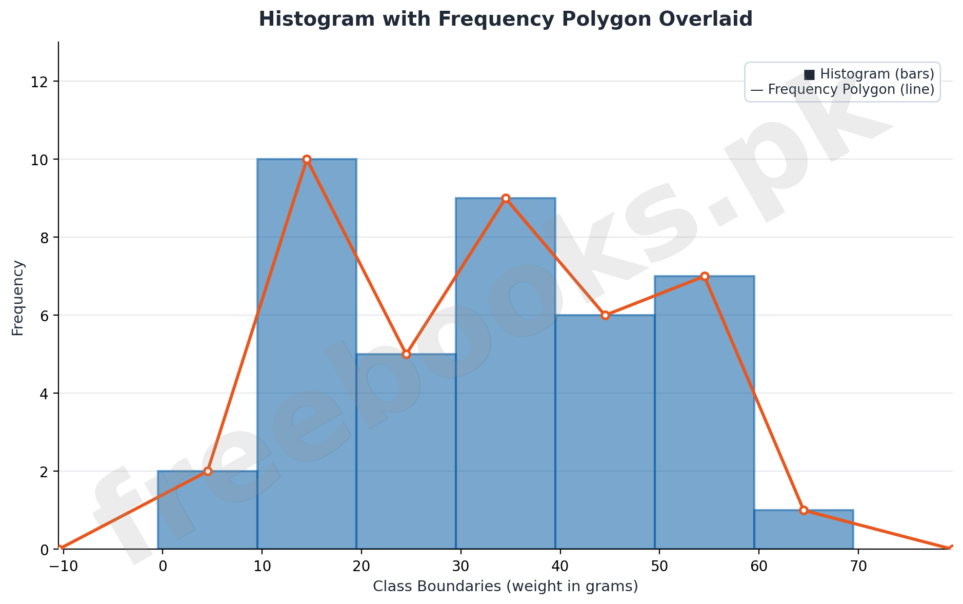
A histogram is a graph of adjacent rectangles built on the XY-plane, with class boundaries marked on the x-axis and frequency on the y-axis; each rectangle's height corresponds to its class's frequency. When all class intervals are equal in size this height is simply the frequency itself. When class intervals are unequal, the raw frequency cannot be used directly — each class's frequency must first be divided by its own class interval size to get a proportional height, so that the AREA of each bar (not just its height) stays proportional to its frequency, keeping the histogram visually honest.

A frequency polygon is a many-sided closed figure formed by plotting a point at each class's midpoint (class mark) against its frequency, then joining consecutive points with straight line segments. To close the figure at both ends, one extra class of the same size is added before the first class and after the last class, each assigned a frequency of zero, so the polygon returns to the x-axis on both sides rather than floating above it.

6.3 Cumulative Frequency Distribution and the Ogive

A cumulative frequency distribution (also called a 'less than' cumulative frequency distribution) is a table showing, against each class's upper class boundary, the running total of all frequencies up to that point. It is built by successively adding each class's frequency to the cumulative total of the classes before it.

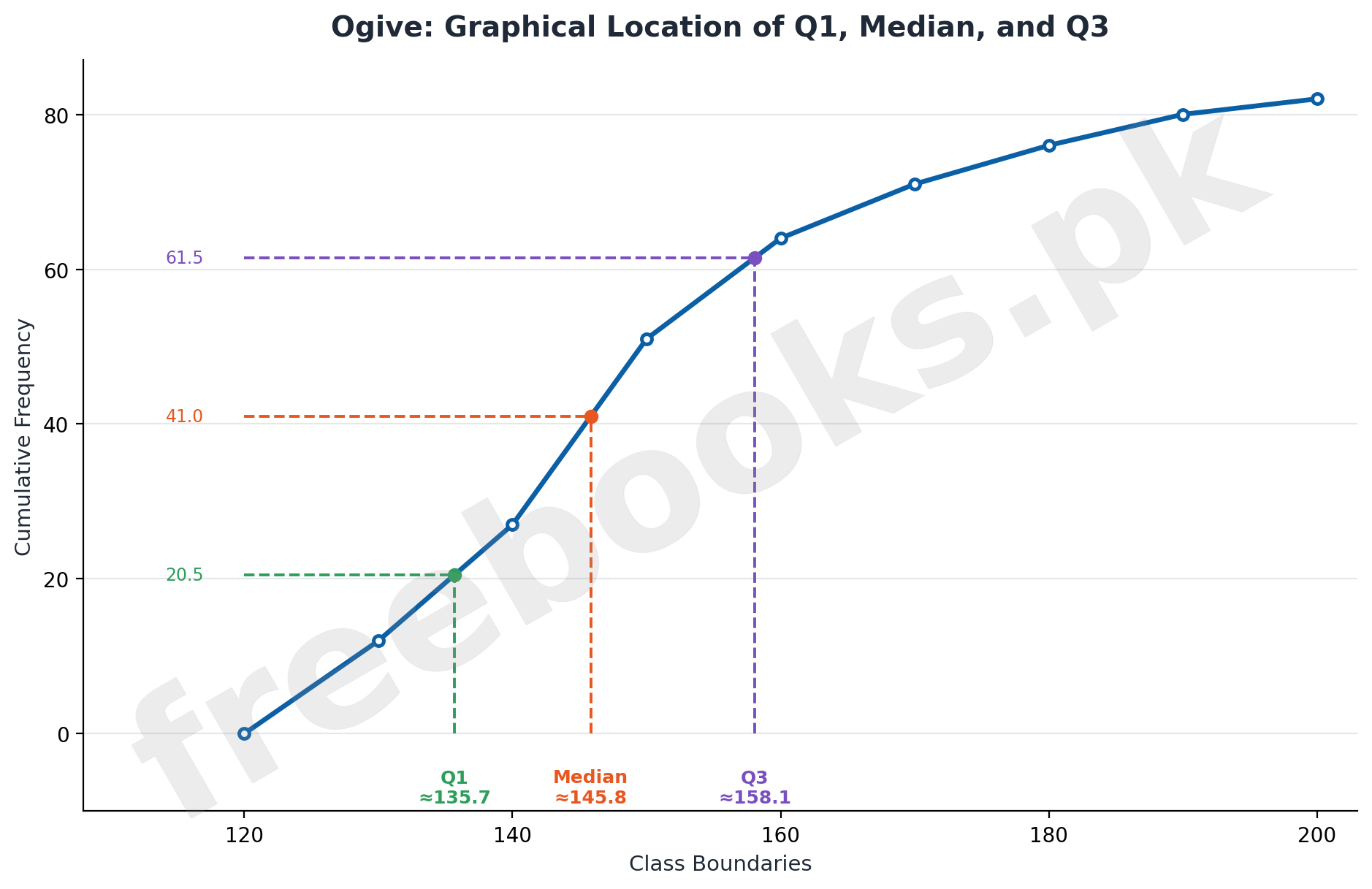
The cumulative frequency polygon, or ogive, is the graph of this cumulative distribution: class boundaries are marked on the x-axis, cumulative frequency on the y-axis, the cumulative frequency at each upper class boundary is plotted as a point, consecutive points are joined by line segments, and a perpendicular is dropped from the final point to the x-axis to close the figure. The ogive's main practical use, covered later in the unit, is reading off the median and quartiles directly from the graph.

6.4 Measures of Central Tendency: Mean, Median, and Mode

The arithmetic mean (X̄) is the sum of all observations divided by their number: X̄ = ΣX/n for ungrouped data, or X̄ = ΣfX/Σf for grouped data (using each class's midpoint X). The indirect (short-cut/coding) method assumes a provisional value A, computes deviations D = X − A (or coded deviations u = D/h), and recovers the true mean as X̄ = A + ΣfD/Σf, or X̄ = A + (Σfu/Σf)×h — useful for simplifying arithmetic with large or awkward values. Four key properties of the mean: the mean of a constant data set is that constant itself; the mean shifts by the same amount as a change of origin (adding a constant to every value adds that constant to the mean); the mean scales the same way as a change of scale (multiplying every value by a constant multiplies the mean by that constant); and the sum of deviations of all observations from their own mean is always exactly zero.

The median is the middle-most observation once data is arranged in order, dividing the data into two equal halves. For ungrouped data with an odd number of observations n, the median is the value at position (n+1)/2; for an even n, it is the average of the values at positions n/2 and (n/2)+1. For grouped discrete data, the median is the value whose cumulative frequency first reaches or passes (n/2). For grouped continuous data, the median class is the class containing the (n/2)th observation (found via cumulative frequency), and the exact median is Median = l + (h/f)(n/2 − c), where l is the median class's lower class boundary, h its class size, f its frequency, and c the cumulative frequency of the class immediately before it. The mode is the most frequently occurring observation — for ungrouped or discrete grouped data it is simply read off directly, while for continuous grouped data the modal class (highest frequency) is located first and then Mode = l + [(fm − f1)/(2fm − f1 − f2)]×h, where fm is the modal class's frequency and f1, f2 are the frequencies of the classes immediately before and after it.

6.5 Geometric Mean, Harmonic Mean, Weighted Mean, and Moving Averages

The geometric mean (G.M.) of n observations is the nth positive root of their product: G.M. = (x1 × x2 × … × xn)^(1/n), most conveniently computed using logarithms as G.M. = Antilog(Σ log X / n) for ungrouped data or Antilog(Σf log X / Σf) for grouped data. The harmonic mean (H.M.) is the reciprocal of the mean of the reciprocals of the observations: H.M. = n / Σ(1/X) for ungrouped data, or H.M. = Σf / Σ(f/X) for grouped data — both are alternative averages used in specific situations (e.g. rates, ratios) where the simple arithmetic mean would be misleading.

The weighted arithmetic mean applies when observations are not all equally important: each value xi is given a weight wi reflecting its relative importance, and the weighted mean is X̄w = Σwx/Σw (compare this to the ordinary mean, which implicitly treats every observation as equally weighted). Moving averages are successive arithmetic means computed over a fixed-size sliding window of consecutive time periods (e.g. a 3-day moving average): the average of the first window is placed at its midpoint, then the window slides forward by dropping the earliest period and adding the next one, repeating until the data is exhausted — this smooths out short-term fluctuations and reveals the underlying trend.

6.6 Graphical Estimation and Measures of Dispersion

The median and quartiles can be located graphically from an ogive: to find the first quartile Q1, locate (n/4) on the y-axis, draw a horizontal line to where it meets the ogive curve, then drop a vertical line down to the x-axis and read the value. The same process applied at 2(n/4) gives the median (Q2), and at 3(n/4) gives the third quartile (Q3). The mode can be located graphically from a histogram: find the tallest rectangle (the modal class), draw a line from its top-left corner to the top-left corner of the next rectangle, another line from its top-right corner to the top-right corner of the previous rectangle, then drop a perpendicular from where these two lines cross down to the x-axis — the point where it meets the x-axis is the mode.

Measures of dispersion describe how spread out or scattered the data is, which is essential because two data sets can share the same mean yet differ greatly in consistency. Range is the simplest measure: Range = Xmax − Xmin for raw data, or (upper class boundary of the last class) − (lower class boundary of the first class) for grouped data. Variance is the mean of the squared deviations from the mean: S² = Σ(X−X̄)²/n for ungrouped data, or S² = ΣfX²/Σf − (ΣfX/Σf)² for grouped data (a computationally faster equivalent form). Standard deviation is simply the positive square root of variance, S = √S² — unlike variance, it is expressed in the same units as the original data, which is why it is the more commonly quoted measure of spread.

Important Definitions

Key Facts and Relations

Topic	Key Fact / Relation
Class size	h = Range / k (k = number of classes)
Class boundary	average of two successive class limits
Class mark (midpoint)	X = (lower limit + upper limit) / 2
Arithmetic mean, direct method (grouped)	X̄ = ΣfX / Σf
Arithmetic mean, indirect method (grouped)	X̄ = A + (Σfu / Σf) × h
Median, grouped continuous data	Median = l + (h/f)(n/2 − c)
Mode, grouped continuous data	Mode = l + [(fm − f1)/(2fm − f1 − f2)] × h
Geometric mean, grouped data	G.M. = Antilog(Σf log X / Σf)
Harmonic mean, grouped data	H.M. = Σf / Σ(f/X)
Weighted mean	X̄w = Σwx / Σw
Range	Range = Xmax − Xmin
Variance and standard deviation, grouped data	S² = ΣfX²/Σf − (ΣfX/Σf)², S = √S²

Diagrams

Histogram with Frequency Polygon: A histogram of adjacent rectangles for a grouped weight distribution, with a frequency polygon line overlaid through the midpoints of each class, closed at both ends with zero-frequency classes

Ogive with Graphical Quartiles: A cumulative frequency polygon (ogive) with dashed guide lines showing how the first quartile, median, and third quartile are read off graphically at n/4, 2n/4, and 3n/4 on the y-axis

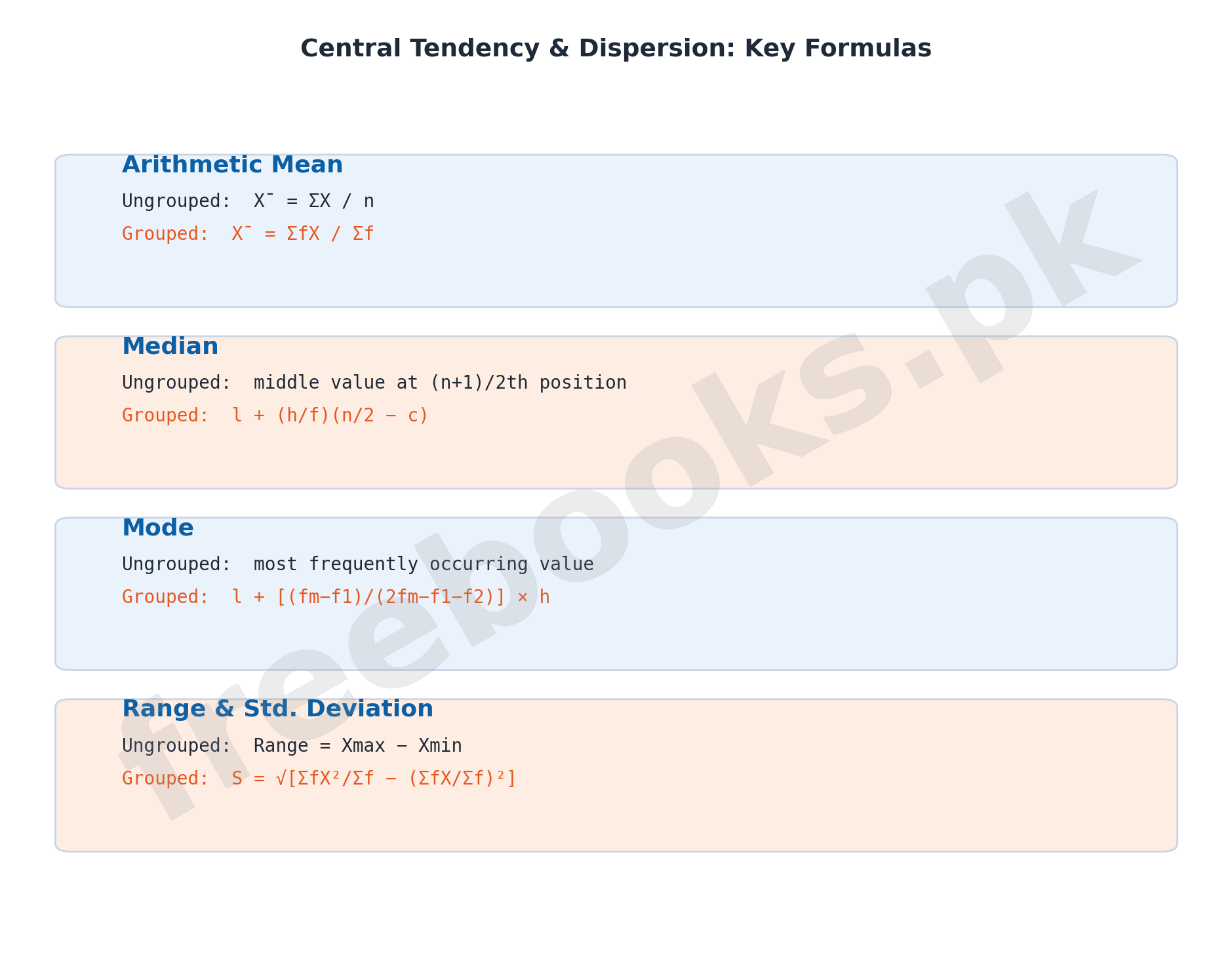
Central Tendency and Dispersion Summary: A summary chart listing the formulas for arithmetic mean, median, mode, and range/standard deviation, for both ungrouped and grouped data

Short Questions & Answers

Long Questions & Answers

Explain how a continuous frequency distribution is constructed, and describe how a histogram and a frequency polygon are drawn from it.

What are the steps in constructing a continuous frequency table?

Find the Range (Xmax − Xmin), choose the number of classes k (usually 5-20, depending on the range), compute the class size h = Range/k (rounding up per the rule of approximation), mark off classes starting from the minimum observation, and tally each observation into its class using tally marks.

What are class limits, class boundaries, and class marks?

Class limits are a class's stated minimum and maximum values; class boundaries are the real limits found by averaging two successive class limits; the class mark (midpoint) is the average of a class's lower and upper limits, used to represent that class in calculations.

How is a histogram constructed for equal class intervals, and how does it differ for unequal intervals?

For equal intervals, class boundaries go on the x-axis and each rectangle's height equals its frequency directly. For unequal intervals, each frequency must first be divided by its own class interval size to get a proportional height, so the bar's AREA (not just height) stays proportional to frequency.

How is a frequency polygon constructed?

Plot each class's midpoint against its frequency, add one zero-frequency class before the first and after the last class to close the figure at both ends, then join all the plotted points with straight line segments.

What is a cumulative frequency table and an ogive?

A cumulative frequency table shows the running total of frequencies up to each class's upper boundary; an ogive is the graph of this table, formed by plotting cumulative frequency against upper class boundaries and joining the points, used later to read off the median and quartiles graphically.

Explain how the mean, median, and mode are calculated for grouped data, and how the measures of dispersion describe the spread of the data.

How is the arithmetic mean calculated for grouped data using the direct and indirect methods?

The direct method uses X̄ = ΣfX/Σf, where X is each class's midpoint. The indirect method assumes a provisional mean A, computes coded deviations u = (X−A)/h, and recovers the true mean as X̄ = A + (Σfu/Σf)×h — useful for simplifying arithmetic with large or awkward class marks.

How is the median located and calculated for grouped continuous data?

First locate the median class — the class whose cumulative frequency first reaches (n/2) — then apply Median = l + (h/f)(n/2 − c), where l is the median class's lower boundary, h its size, f its frequency, and c the cumulative frequency of the class before it.

How is the mode calculated for grouped continuous data?

Locate the modal class (the class with the highest frequency fm), note the frequencies f1 and f2 of the classes immediately before and after it, then apply Mode = l + [(fm−f1)/(2fm−f1−f2)]×h, where l is the modal class's lower boundary and h its size.

What is the range, and how is it defined for grouped data?

Range is the simplest measure of dispersion: for raw data it is Xmax − Xmin; for grouped data it is the upper class boundary of the last class minus the lower class boundary of the first class.

What do variance and standard deviation measure, and how are they calculated?

Variance is the mean of the squared deviations of observations from their mean, S² = Σ(X−X̄)²/n (or the computational form ΣfX²/Σf − (ΣfX/Σf)² for grouped data); standard deviation S = √S² is its square root, expressed in the original data's units, and is used to compare how consistent or spread out two data sets are even when they share the same mean.

Multiple Choice Questions (MCQs)

Quick Revision Summary

• Frequency distribution: tabular grouping of data with frequency per group | grouped data = data in this form
• Class size h = Range/k | Class boundary = average of two successive class limits | Class mark = (lower+upper limit)/2
• Cumulative frequency: running total of frequencies up to a class's upper boundary
• Histogram: adjacent rectangles on class boundaries, height = frequency (or proportional height for unequal intervals)
• Frequency polygon: line through class-mark/frequency points, closed with zero-frequency classes at both ends
• Ogive: graph of the cumulative frequency distribution; used to read median/quartiles graphically
• Arithmetic mean: X̄ = ΣfX/Σf (direct) or A + (Σfu/Σf)×h (indirect/short-cut)
• Mean properties: constant data → mean = constant | shifts with origin change | scales with scale change | Σ(X−X̄) = 0
• Median (grouped continuous) = l + (h/f)(n/2 − c) | Mode (grouped continuous) = l + [(fm−f1)/(2fm−f1−f2)]×h
• Geometric mean = Antilog(Σf log X/Σf) | Harmonic mean = Σf/Σ(f/X) | Weighted mean = Σwx/Σw
• Moving average: successive means over a sliding window of fixed size, smooths short-term fluctuation
• Range = Xmax−Xmin | Variance S² = ΣfX²/Σf − (ΣfX/Σf)² | Standard deviation S = √S²

Exam Tips

• Always compute class boundaries before finding class marks or plotting a histogram — mixing up limits and boundaries is the most common calculation error in this unit
• For unequal-interval histograms, remember to divide frequency by class interval size first — skipping this step distorts the shape of the whole histogram
• When finding the median or mode for grouped data, locate the correct class FIRST using cumulative frequency, then plug values into the formula — never guess the class
• Use the indirect (assumed mean) method whenever raw values are large or awkward — it gives the exact same answer as the direct method with far less arithmetic
• On an ogive, always work in the same order: locate n/4, 2n/4, 3n/4 on the y-axis, draw horizontal then vertical guide lines, and read the x-axis value
• Remember variance is in squared units of the data (e.g. sq. gm) while standard deviation is back in the original units — always take the square root before comparing spread across two data sets