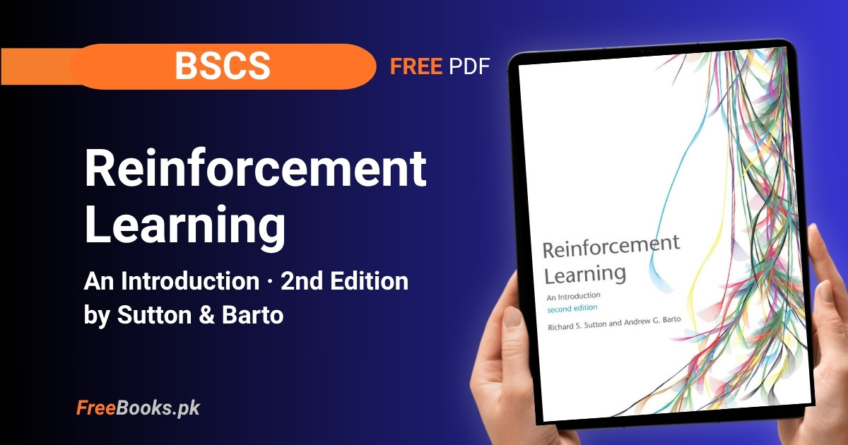
BSCS and MS students studying Reinforcement Learning can read the complete second edition of “Reinforcement Learning: An Introduction” by Richard S. Sutton and Andrew G. Barto free online at its official site, hosted by the authors themselves. Published by MIT Press in 2018 (with a corrected printing in 2020, per the book’s own copyright page), it is the book almost every Reinforcement Learning course, in Pakistan and internationally, treats as the standard reference — not because it is the newest book on the subject, but because Sutton and Barto helped define reinforcement learning as a field, and this is the text where its core ideas (value functions, temporal-difference learning, policy gradients) were first laid out clearly enough for a full course to be built around them.
Its structure moves deliberately from simple to hard. Part I (Chapters 2-8) develops as much of reinforcement learning as possible in the tabular case, where exact solutions exist — multi-armed bandits, Markov decision processes, dynamic programming, Monte Carlo methods, temporal-difference learning, n-step bootstrapping, and planning with a learned model. Part II (Chapters 9-13) extends the same ideas to function approximation, ending with policy gradient methods. Part III (Chapters 14-17) steps back from algorithms to reinforcement learning’s connections to psychology and neuroscience, real applications like AlphaGo and TD-Gammon, and open research frontiers. There is no runnable code in the book itself, only pseudocode boxes, which is exactly why it works so well as the theory companion to a hands-on, code-first course project.
Book Overview
| Course | Reinforcement Learning (Computer Science elective) |
| Degree Programs | BSCS (also very commonly used as the standard MS-level Machine Learning / Reinforcement Learning course text) |
| Level | University / Advanced undergraduate and graduate |
| Edition | 2nd Edition, MIT Press (2018; corrected printing 2020) |
| Author(s) | Richard S. Sutton, Andrew G. Barto |
| Publisher | MIT Press (Adaptive Computation and Machine Learning series) |
| Structure | 17 chapters in three parts (I: Tabular Solution Methods; II: Approximate Solution Methods; III: Looking Deeper), plus references and index |
| License | Creative Commons Attribution-NonCommercial-NoDerivs 2.0 Generic (CC BY-NC-ND 2.0), stated on the book’s own copyright page |
| Language | English |
| Format | Free official PDF (full book, plus a margin-trimmed edition), hosted directly by the authors |
Chapter List
Chapter 1: Introduction
Difficulty: Easy · Key topics: trial-and-error learning, delayed reward, evaluative vs instructive feedback, elements of RL, tic-tac-toe example, three historical threads
Chapter 1 defines reinforcement learning as learning what to do — how to map situations to actions — so as to maximize a numerical reward signal, discovered by trying actions rather than being told the correct one. It names trial-and-error search and delayed reward as the field’s two most important distinguishing features, and positions RL as a third machine learning paradigm alongside supervised and unsupervised learning. The chapter previews the four elements of an RL system (policy, reward signal, value function, and an optional model), works through a tic-tac-toe example that anticipates Chapter 6’s temporal-difference method, and closes with a detailed history tracing three threads — trial-and-error learning, optimal control, and temporal-difference learning — that fully merged only with Watkins’s 1989 Q-learning.
Key Points:
- RL is defined as learning what to do, mapping situations to actions, to maximize a numerical reward signal — the learner discovers good actions by trying them, it is not told them directly.
- Trial-and-error search and delayed reward are named the two most important distinguishing features of reinforcement learning.
- RL is described as a third machine learning paradigm, distinct from supervised learning (learns from labeled examples of correct behavior) and unsupervised learning (finds hidden structure in unlabeled data).
- The problem is formalized as the optimal control of an incompletely-known Markov decision process, worked out in full in Chapter 3.
- Four elements of an RL system are named: a policy, a reward signal, a value function, and, optionally, a model of the environment used for planning.
- The chapter traces three historical threads — trial-and-error learning, optimal control/dynamic programming, and temporal-difference learning — that came together fully only with Watkins’s Q-learning in 1989.
Memory Tip: Remember “the two most important features” as a pair: trial-and-error (you have to try actions to learn their value) plus delayed reward (an action’s payoff may not show up until many steps later).
Common Mistake: Treating reinforcement learning as a loose synonym for “any algorithm that uses rewards.” The chapter’s actual distinction is sharper: RL is specifically about learning from evaluative feedback (how good was the action taken) rather than instructive feedback (what was the correct action) — and it is that distinction, not the mere presence of a reward, that makes exploration necessary.
Important Questions:
- What are the two most important distinguishing features of reinforcement learning? Trial-and-error search and delayed reward — the learner must discover good actions by trying them, and an action can affect rewards many steps in the future, not just the next one.
- What are the four main elements of a reinforcement learning system? A policy (mapping states to actions), a reward signal (the goal, received each step), a value function (long-term desirability of states), and, optionally, a model of the environment used for planning.
Chapter 2: Multi-armed Bandits
Part 1: Tabular Solution Methods · Difficulty: Medium · Key topics: k-armed bandit, action-value methods, epsilon-greedy, incremental updates, nonstationary problems, optimistic initial values, UCB, gradient bandits, contextual bandits
This chapter isolates the exploration/exploitation tradeoff in the simplest possible setting: repeatedly choosing among k actions, each with a fixed but unknown expected reward (its “value”), to maximize total reward over time. It introduces sample-average action-value estimates and epsilon-greedy selection, then turns the averaging update into an efficient incremental rule and extends it to nonstationary bandits with a constant step size. It compares optimistic initial values, Upper-Confidence-Bound (UCB) action selection, and gradient bandit algorithms based on a soft-max preference update, before closing on associative search (contextual bandits) — a first step toward choosing different actions in different situations.
Key Points:
- The true value of action a,
q*(a), is the expected reward given that a is selected; the agent maintains an estimateQ_t(a)and tries to keep it close toq*(a). - Choosing the action with the current highest estimated value is “exploiting”; choosing a different action to improve its estimate is “exploring” — the two cannot both happen on a single step.
- The incremental update rule
NewEstimate = OldEstimate + StepSize × (Target − OldEstimate)recovers the sample average with step size1/n, without storing every past reward. - A constant step size (instead of
1/n) is needed to track a nonstationary bandit, because it weights recent rewards more heavily and never fully forgets. - Optimistic initial values push early exploration for free, by making every untried action look better than its eventual true value, but the trick only helps temporarily and not at all in nonstationary problems.
- UCB action selection adds an uncertainty bonus that shrinks as an action is tried more often, favoring actions that could plausibly be optimal rather than exploring uniformly at random.
- Gradient bandit algorithms learn a numerical preference for each action via stochastic gradient ascent and convert preferences to probabilities with a soft-max distribution, rather than estimating action values at all.
Practice Tip: Implement the 10-armed testbed yourself and run epsilon-greedy with a few different epsilon values (0, 0.01, 0.1) over 1000 steps, averaged over many runs — watching greedy (epsilon = 0) get permanently stuck on a suboptimal action is the clearest illustration in the whole book of why exploration matters.
Common Mistake: Assuming a bigger epsilon (more exploration) is always better. In the 10-armed testbed, epsilon = 0.1 explores more but settles on a lower average reward in the long run than epsilon = 0.01, because it keeps selecting known-worse actions 10% of the time forever — the right amount of exploration depends on reward variance and time horizon, not just “more caution is safer.”
Important Questions:
- Why does a constant step size suit nonstationary bandit problems better than the sample-average method? The sample-average method weights all past rewards equally, so it adapts more and more slowly to a moving target; a constant step size gives exponentially more weight to recent rewards, so it keeps tracking a target that keeps changing.
- How does UCB action selection decide which non-greedy action to try? It adds an uncertainty term that grows with time and shrinks each time that action is selected, favoring actions that are either promising or under-explored, rather than exploring uniformly at random the way epsilon-greedy does.
Chapter 3: Finite Markov Decision Processes
Part 1: Tabular Solution Methods · Difficulty: Medium · Key topics: agent-environment interface, return, episodic vs continuing tasks, policies, state/action-value functions, Bellman equation, optimal policies, Bellman optimality equation
This chapter formalizes the full reinforcement learning problem as a finite Markov decision process (MDP). The agent and environment interact at discrete time steps: the agent observes a state, selects an action, and one step later receives a reward and a new state, all governed by a single dynamics function p(s',r|s,a). It defines the return as a (possibly discounted) sum of future rewards, distinguishes episodic from continuing tasks, and defines the state-value function v_pi(s) and action-value function q_pi(s,a) for a given policy, each satisfying a recursive Bellman equation relating a state’s value to its successors’ values. It closes by defining the optimal value functions v* and q* and the Bellman optimality equations they satisfy.
Key Points:
- The dynamics function
p(s',r|s,a)fully characterizes the environment, giving the joint probability of the next state and reward given the current state and action. - The return
G_tis the (discounted) sum of future rewards the agent tries to maximize; the discount rate gamma between 0 and 1 trades off immediate versus future reward. - A policy
pi(a|s)is a probability distribution over actions for each state;v_pi(s)is the expected return starting from s and following pi. - The Bellman equation expresses a state’s value recursively as the expected immediate reward plus the discounted value of the next state, averaged over the policy and the environment’s dynamics.
- An optimal policy has a value function
v*(s)at least as large as every other policy’s value function, for every state simultaneously; every finite MDP has at least one such policy. - The Bellman optimality equation replaces the average-over-actions in the ordinary Bellman equation with a max over actions, since an optimal policy always selects the highest-value action.
- Once
v*is known, any policy that is greedy with respect to it is automatically an optimal policy.
Memory Tip: Read the Bellman equation as “today’s value = today’s expected reward + tomorrow’s (discounted) value,” applied at every state — nearly every value-based method in the rest of the book is some way of turning this one recursive relationship into a workable update rule.
Common Mistake: Confusing the state-value function v_pi(s) with the action-value function q_pi(s,a). v_pi(s) is the value of being in a state and then following pi; q_pi(s,a) is the value of taking a specific action in that state and following pi afterward — an agent needs q, not v, to select actions without also having a model of the environment.
Important Questions:
- What is the difference between an episodic task and a continuing task? An episodic task has a natural terminal state after which the interaction resets (a game, a maze run); a continuing task has no terminal state and goes on indefinitely, which is why the book relies on discounting — an undiscounted sum of infinitely many rewards could otherwise be infinite.
- How does the Bellman optimality equation for v* differ from the ordinary Bellman equation for a fixed policy? The ordinary equation averages the expected next value over the policy’s action probabilities; the optimality equation instead takes the maximum over actions, because an optimal policy always picks the single best action rather than following a fixed distribution.
Chapter 4: Dynamic Programming
Part 1: Tabular Solution Methods · Difficulty: Medium · Key topics: policy evaluation, policy improvement, policy iteration, value iteration, asynchronous DP, generalized policy iteration
Dynamic programming (DP) is a collection of algorithms that compute optimal policies given a perfect model of the environment as a finite MDP — of limited direct use in RL because of that model requirement, but foundational because every later method in the book can be seen as trying to achieve DP’s same effect with less computation. The chapter develops iterative policy evaluation, which repeatedly applies the Bellman equation as an update rule until convergence, then policy improvement, which shows that acting greedily with respect to a policy’s value function produces an equal-or-better policy. Alternating the two gives policy iteration; folding them into one sweep gives value iteration. It closes with asynchronous DP and generalized policy iteration (GPI), the near-universal pattern of two interacting processes making a value function consistent with a policy and a policy greedy with respect to a value function.
Key Points:
- DP requires a perfect model of the environment’s dynamics; later RL methods relax this requirement but reuse DP’s core update ideas.
- Iterative policy evaluation turns the Bellman equation for
v_piinto an update rule, sweeping through all states repeatedly until the values stop changing significantly. - The policy improvement theorem: acting greedily with respect to
v_piin every state produces a policy at least as good as pi, and strictly better unless pi was already optimal. - Policy iteration alternates complete policy evaluation with policy improvement and is guaranteed to converge to an optimal policy in a finite number of iterations for a finite MDP.
- Value iteration truncates evaluation to a single sweep before each improvement step, combining both into one update and usually converging faster in practice.
- Generalized Policy Iteration (GPI) is the general pattern — two processes, one for value consistency and one for policy greediness, interacting toward optimality — that nearly every algorithm in the book turns out to be a variation of.
- Asynchronous DP updates states in any order, possibly skipping some many times before touching others, which can speed convergence when combined with a good ordering.
Memory Tip: GPI is the one idea worth memorizing from this chapter — two arrows pointing at each other, “value consistent with policy” and “policy greedy with respect to value,” converging toward the point where both arrows agree; most later algorithms are a different way of implementing this same interaction.
Common Mistake: Assuming DP methods “learn” from experience the way the rest of the book’s methods do. DP computes exact value functions from a known model through full sweeps of every state — no environment interaction or sampling is involved, which is exactly why Chapter 5 introduces Monte Carlo methods for the case where the model is unknown.
Important Questions:
- What is the difference between policy iteration and value iteration? Policy iteration runs policy evaluation to convergence before each improvement step; value iteration performs just one evaluation sweep before improving the policy again, trading evaluation accuracy per iteration for typically faster overall convergence.
- What is generalized policy iteration (GPI)? The general pattern of two interacting processes — one making the value estimate consistent with the current policy, the other making the policy greedy with respect to the current value estimate — that together converge toward the optimal value function and policy; nearly every algorithm in the rest of the book is recognizable as a variation of this interaction.
Chapter 5: Monte Carlo Methods
Part 1: Tabular Solution Methods · Difficulty: Medium · Key topics: episodic tasks, first-visit vs every-visit MC, MC prediction, MC control, exploring starts, off-policy prediction, importance sampling
Monte Carlo (MC) methods estimate value functions and discover optimal policies purely from sample experience — episodes of states, actions and rewards — without requiring any knowledge of the environment’s dynamics, unlike DP. Because MC needs a well-defined return, it is defined here only for episodic tasks, updating value estimates once an episode completes by averaging observed returns (first-visit and every-visit MC are both introduced). The chapter adapts generalized policy iteration to this setting: learn q instead of v so action selection needs no model, and keep every state-action pair being visited, either through “exploring starts” or through soft policies that never become fully greedy. It closes on off-policy prediction, learning about a target policy from a different behavior policy’s experience using importance sampling to correct for the mismatch.
Key Points:
- Monte Carlo methods learn purely from sample episodes of experience, requiring no model of the environment’s transition probabilities.
- First-visit MC averages the return following only the first visit to a state per episode; every-visit MC averages returns after every visit; both converge to
v_pibut have different theoretical properties. - Because only complete episodes produce a well-defined return, MC updates happen episode-by-episode, not step-by-step, and MC as presented here is defined only for episodic tasks.
- MC methods learn action values
q_pi(s,a)rather than state values for control, because selecting actions from v alone would require a model to look one step ahead. - The exploring-starts assumption — every state-action pair has a nonzero chance of starting an episode — guarantees every action gets tried, but is often unrealistic in practice.
- On-policy MC control with soft (e.g. epsilon-soft) policies replaces exploring starts by never letting the policy become fully deterministic.
- Off-policy MC prediction learns the target policy’s value from behavior-policy episodes using the importance-sampling ratio, the product of the two policies’ action-probability ratios, to reweight each return correctly.
Memory Tip: Contrast MC with DP in one sentence: DP computes value functions by sweeping over every possible transition using a known model; MC estimates the same functions by averaging the actual returns that show up in sampled episodes — no model, no sweep, just experience and arithmetic.
Common Mistake: Applying a Monte Carlo update in the middle of an episode. The return G_t is only known once the episode terminates, so every MC update must wait until the episode ends, unlike the step-by-step updates in Chapter 6 — trying to update mid-episode with an incomplete return is a common implementation bug.
Important Questions:
- Why must Monte Carlo methods wait until an episode ends before updating any value estimate? An MC update is based on the actual observed return, the total discounted reward from that time step until the episode terminates, which cannot be computed until the episode actually ends — so every update happens episode-by-episode, not step-by-step.
- Why does Monte Carlo control usually learn action values q(s,a) rather than state values v(s)? Choosing an action from v(s) alone would require looking one step ahead with a model of the environment; because MC methods have no model, they need q(s,a) directly, so the agent can compare actions in a state without knowing what each one leads to.
Chapter 6: Temporal-Difference Learning
Part 1: Tabular Solution Methods · Difficulty: Medium · Key topics: TD(0), bootstrapping, Sarsa, Q-learning, Expected Sarsa, maximization bias, double learning
Temporal-difference (TD) learning is presented as the single idea most central and novel to reinforcement learning, combining Monte Carlo’s ability to learn directly from raw experience with dynamic programming’s bootstrapping — updating an estimate based partly on other learned estimates rather than waiting for a final outcome. TD(0) updates V(S_t) toward R_(t+1) + gamma·V(S_(t+1)) immediately after each transition, instead of waiting for the full return as Monte Carlo does. The chapter builds Sarsa (on-policy TD control, using the action actually taken next), Q-learning (off-policy TD control, using the best possible next action regardless of what is actually taken), and Expected Sarsa (averaging over all next actions). It closes by identifying maximization bias, the systematic overestimation that occurs whenever a max over noisy estimates both selects and evaluates an action, with double learning as the fix.
Key Points:
- TD(0) updates
V(S_t)towardR_(t+1) + gamma·V(S_(t+1))as soon as the next reward and state are observed, without waiting for the episode to end. - TD methods are called bootstrapping methods because, like DP but unlike Monte Carlo, they base an update partly on an existing estimate rather than only on actual sampled reward.
- Sarsa is on-policy: it updates
Q(S,A)using the actual next action chosen by the current policy, so the policy being learned and the policy generating behavior are the same. - Q-learning is off-policy: it updates
Q(S,A)using the maximum Q-value over all possible next actions, regardless of which action is actually taken next, learning the optimal policy while behaving differently (e.g. exploring). - Expected Sarsa replaces Sarsa’s sampled next action with the expectation over all next actions weighted by the policy, reducing variance at extra computational cost.
- Maximization bias occurs because the same noisy value estimates are used both to select the best-looking action and to evaluate it, systematically inflating value estimates.
- Double learning fixes this by maintaining two independent value estimates — one selects the greedy action, the other evaluates it — alternating which is updated.
Practice Tip: Implement Sarsa and Q-learning on a Cliff Walking gridworld and compare the learning curves directly — Q-learning learns the optimal (risky, along-the-cliff) path faster, but Sarsa’s online performance during training is actually better because it accounts for the exploratory policy’s occasional falls, a concrete illustration of the on-policy/off-policy distinction.
Common Mistake: Assuming Q-learning always outperforms Sarsa because it learns the optimal policy. Q-learning learns the value of the optimal policy, but actual behavior during training (still epsilon-greedy) can perform worse online than Sarsa’s more cautious, policy-aware behavior — “learns the better policy” and “performs better while learning” are not the same claim.
Important Questions:
- What is the key difference between Sarsa and Q-learning? Sarsa is on-policy — it updates using the actual next action selected by the current behavior policy — while Q-learning is off-policy, updating using the maximum Q-value over all possible next actions and learning the value of the greedy policy regardless of the exploratory actions actually taken.
- What causes maximization bias, and how does double learning correct it? A max operator applied to noisy value estimates tends to select the estimate that happens to be too high, systematically overestimating true values; double learning keeps two separate estimates, using one to choose the greedy action and the other to evaluate it, so the same noisy estimate is never used for both roles.
Chapter 7: n-step Bootstrapping
Part 1: Tabular Solution Methods · Difficulty: Medium · Key topics: n-step return, n-step TD, n-step Sarsa, n-step off-policy learning, tree backup, tyranny of the time step
This chapter unifies Monte Carlo and one-step TD by generalizing to n-step updates, which use the next n rewards plus the estimated value n steps ahead as the update target — one-step TD at n = 1, Monte Carlo as n approaches infinity. It shows how n-step methods free the learner from “the tyranny of the time step,” in which one-step TD’s single time interval must do double duty as both the action-selection interval and the bootstrapping interval, a compromise n-step methods avoid. The chapter extends n-step prediction to n-step Sarsa for control, then to n-step off-policy learning via importance sampling, and to the n-step tree-backup algorithm, which needs no importance sampling because it backs up from the estimated value of every possible action, not just the one taken.
Key Points:
- An n-step return sums the next n actual rewards and adds the discounted estimated value of the state reached n steps later; one-step TD is n = 1 and Monte Carlo is the n = infinity limit.
- n-step methods are still TD methods (they bootstrap from a later estimate), just with that later estimate n steps ahead instead of one.
- The best-performing n in practice is usually neither the smallest nor the largest — intermediate n often beats both one-step TD and full Monte Carlo.
- n-step Sarsa extends the idea to action values for on-policy control, using the actual n-step sequence of actions taken.
- n-step off-policy learning corrects for the target/behavior policy mismatch with an importance-sampling ratio, but the ratio’s variance grows rapidly with n.
- The n-step tree-backup algorithm avoids importance sampling entirely, backing up from the estimated values of all actions (taken or not) weighted by the target policy’s probabilities.
- n-step methods are introduced partly as a bridge to eligibility traces (Chapter 12), which achieve a similar TD/Monte Carlo spectrum more efficiently.
Memory Tip: Picture the backup diagrams as a ladder: one-step TD backs up after 1 reward, Monte Carlo backs up only after the whole episode, and n-step methods are every rung in between — bigger n means “wait longer before updating, but trust the bootstrap estimate less.”
Common Mistake: Assuming a larger n is strictly “more accurate.” A larger n does reduce bias from bootstrapping, but it also increases variance, since more random rewards get summed into a single target — intermediate n values typically beat both extremes, not the largest n.
Important Questions:
- What is “the tyranny of the time step” that n-step methods escape? With one-step TD, the same fixed interval must serve two roles — how often the agent can act, and how far ahead it bootstraps — even though the best interval for each is often different; n-step methods decouple the two by letting the bootstrapping horizon (n) be chosen independently.
- How does n-step tree-backup achieve off-policy learning without importance sampling? Instead of correcting a sampled action’s target with a probability ratio, it computes an expected update at every step over all actions, taken or not, weighted by the target policy’s own probabilities, so no “how likely was the behavior policy to pick this action” correction is ever needed.
Chapter 8: Planning and Learning with Tabular Methods
Part 1: Tabular Solution Methods · Difficulty: Medium · Key topics: distribution vs sample models, Dyna-Q, prioritized sweeping, expected vs sample updates, Monte Carlo Tree Search
This chapter unifies model-based methods (which rely on planning from a model, like DP) and model-free methods (which rely on learning from real experience, like Monte Carlo and TD), showing both compute value functions the same underlying way — by backing up simulated or real experience into an update target. Dyna-Q integrates planning, acting and learning in one architecture: it learns a model from real experience, uses that model to generate simulated experience, and applies the same Q-learning update to both real and simulated transitions. The chapter covers what happens when the learned model is wrong (and how exploration bonuses correct for it), prioritized sweeping (focusing computation on states whose values recently changed most), expected versus sample updates, and closes with heuristic search, rollout algorithms and Monte Carlo Tree Search, the planning method behind AlphaGo.
Key Points:
- A distribution model produces every possible next state/reward and its probability; a sample model produces just one, sampled according to the true probabilities — sample models are often much easier to build.
- Planning is defined broadly as any computational process that takes a model as input and produces or improves a policy.
- Dyna-Q performs one step of real Q-learning per real environment interaction, then several additional Q-learning updates using simulated transitions from a learned model, using the identical update rule for both.
- When a learned model becomes inaccurate, an exploration bonus that rewards visiting long-untried states (Dyna-Q+) helps the agent rediscover the change.
- Prioritized sweeping maintains a priority queue of states ranked by how much their value estimate recently changed, focusing computation where it will most likely help.
- An expected update considers all possible next states weighted by probability; a sample update uses just one sampled next state — cheaper per update, and often more efficient overall for a fixed computational budget.
- Monte Carlo Tree Search plans at decision time by repeatedly simulating from the current state and using the outcomes to pick the actual action — the planning method behind AlphaGo and AlphaGo Zero (Chapter 16).
Practice Tip: Implement basic Dyna-Q on a small gridworld and vary the planning-steps parameter n (simulated updates per real step) from 0 upward — watching how quickly the number of real steps needed to solve the maze drops as n increases is the clearest demonstration in the book of what planning with a learned model actually buys you.
Common Mistake: Assuming more planning steps in Dyna-Q are always better once the model is learned. If the environment can change (a shortcut opens, a wall appears), a purely greedy Dyna-Q agent can keep exploiting its now-stale model indefinitely; Dyna-Q+’s exploration bonus exists specifically because more planning without renewed exploration can make an agent worse when the world changes.
Important Questions:
- What is the core idea of the Dyna-Q architecture? Dyna-Q learns a model from real experience and treats simulated transitions from that model exactly the same as real transitions, applying the same Q-learning update to both, so one real step of experience can drive many additional updates through planning without any new environment interaction.
- Why can sample updates make more overall progress than expected updates for the same computation? An expected update accounts for every possible next state exactly but costs proportional to the branching factor, whereas a sample update uses one sampled transition at a fraction of the cost; the larger number of cheaper, noisier updates this allows often reduces error faster overall, especially when the branching factor is large.
Chapter 9: On-policy Prediction with Approximation
Part 2: Approximate Solution Methods · Difficulty: Hard · Key topics: function approximation, Value Error objective, semi-gradient methods, linear methods, tile coding, Fourier basis, neural networks, least-squares TD
This chapter opens Part II by moving from tabular value functions to approximate ones, representing v_pi(s) as a parameterized function of a weight vector w — linear in features, a neural network, or a decision tree — instead of one entry per state. Because the number of weights is typically far smaller than the number of states, updating one state’s estimate generalizes and changes the estimated values of many other states at once. The chapter defines the Value Error (VE) objective, weighted by how often each state is actually visited, and derives semi-gradient methods (so called because the bootstrapping target itself depends on the weights being updated, and the gradient deliberately ignores that dependency), including semi-gradient TD(0). It surveys linear methods and feature construction — polynomials, the Fourier basis, coarse coding, tile coding, radial basis functions — before touching artificial neural networks and least-squares TD.
Key Points:
- Function approximation represents the estimated value as
v-hat(s,w), a parameterized function with weight vector w whose dimension is typically much smaller than the number of states. - Because the weight vector is much smaller than the state space, updating one state’s estimate generalizes and changes the estimated values of many other states — powerful, but harder to reason about than a lookup table.
- The Value Error objective weights the squared error at each state by how often that state is actually visited under the policy, not uniformly across all states.
- Semi-gradient methods treat the bootstrapping target as fixed when computing the gradient, even though it depends on the same weights being updated — efficient and usually effective, but not true gradient descent.
- Linear methods represent
v-hatas a dot product of a weight vector and a feature vector; their convergence properties are the best understood of any function approximation method in the book. - Tile coding partitions the state space into multiple overlapping offset grids, giving coarse coding’s generalization benefits with efficient, sparse, binary features well suited to online learning.
- Feature construction — which features to compute from the raw state — is often more important to a linear method’s success in practice than the learning algorithm chosen.
Memory Tip: The word “semi” in semi-gradient is the whole idea worth remembering: the target used in the update depends on the same weights being updated, and the method deliberately ignores that dependency — which is why these methods, unlike true stochastic gradient descent, are not guaranteed to converge in every case, even though they usually work well.
Common Mistake: Assuming that giving a linear function approximator more features can only help. More features mean more weights and a harder-to-fit approximation, and with sparse or noisy data more features can hurt generalization — the whole discussion of tile coding, coarse coding and the Fourier basis is about choosing features economically, not maximizing their count.
Important Questions:
- Why are semi-gradient methods called “semi” rather than true gradient methods? The update target for semi-gradient TD(0) itself depends on the same weight vector being updated; a true gradient-descent method would differentiate through that dependency too, but semi-gradient methods deliberately treat the target as fixed and take the gradient only of the current estimate, which is simpler and usually works but loses true SGD’s convergence guarantees.
- What problem does tile coding solve, and how does it work? It builds informative, generalizing features from a continuous state space cheaply enough for online learning, by overlaying several offset grids (“tilings”) so a state’s feature vector marks exactly one active tile per tiling — nearby states share most active tiles (generalizing between them) while distant states share none.
Chapter 10: On-policy Control with Approximation
Part 2: Approximate Solution Methods · Difficulty: Hard · Key topics: episodic semi-gradient Sarsa, Mountain Car, average reward setting, differential value functions, deprecating discounting
This chapter extends function approximation from prediction to control, introducing episodic semi-gradient Sarsa, the natural extension of semi-gradient TD(0) to action values, paired with epsilon-greedy for policy improvement. It works through the Mountain Car task — an underpowered car that must build momentum by first moving away from the goal — as the running example for semi-gradient Sarsa and n-step Sarsa with tile-coded features. The chapter then turns to continuing tasks and argues that once genuine function approximation is used, the usual discounted-reward setting stops being a sound way to define an optimal policy, so it switches to an average-reward formulation with new “differential” value functions that measure value relative to the long-run average reward rate, not a discounted sum.
Key Points:
- Episodic semi-gradient Sarsa extends semi-gradient TD(0) to action-value approximation
q-hat(s,a,w), coupled with epsilon-greedy for on-policy control. - The Mountain Car task requires the agent to first drive away from the goal, up the opposite slope, to build enough momentum, since the engine alone cannot overcome gravity on the direct route.
- With tabular methods, average-reward and discounted-reward optimal policies always coincide in the continuing case; this chapter shows the equivalence breaks down once function approximation is introduced.
- The average reward rate is the long-run average reward per time step under a policy; differential return replaces the discounted sum with the sum of deviations from this average.
- Differential value functions measure a state’s or action’s value relative to the average reward rate, rather than as an absolute discounted quantity.
- Differential semi-gradient Sarsa maintains a running estimate of the average reward alongside the value-function weights, using it directly in its TD-error update.
- The chapter recommends deprecating the discounted setting for continuing problems with function approximation specifically — discounting remains sound for episodic problems.
Practice Tip: Implement semi-gradient Sarsa with tile coding on Mountain Car and watch the steps-to-goal per episode fall over the first few hundred episodes, then try a poor tiling resolution and see how much feature design, not just the learning algorithm, determines whether the car solves the task at all.
Common Mistake: Assuming discounting still “just works” for continuing tasks once function approximation is added, the way it does in the tabular case. This chapter shows explicitly that under function approximation, maximizing discounted return in a continuing task is not equivalent to maximizing average reward — this is exactly why it formally recommends the average-reward, differential-value formulation for continuing tasks with approximation.
Important Questions:
- What makes the Mountain Car task hard, and why is it a good example for semi-gradient Sarsa? The car’s engine cannot drive directly up the goal slope from a standing start, so the only solution is to first drive backward to build momentum; the continuous state space also forces the use of function approximation (tile coding here) rather than a lookup table.
- Why does the chapter argue for abandoning discounting in continuing tasks once function approximation is used? Under function approximation, maximizing discounted return in a continuing task no longer necessarily maximizes the true long-run average reward the way it always does in the tabular case, so the chapter instead defines an average-reward objective and differential value functions that remain sound under approximation.
Chapter 11: *Off-policy Methods with Approximation
Part 2: Approximate Solution Methods · Difficulty: Hard (marked with an asterisk in the book itself as more advanced/optional material) · Key topics: semi-gradient off-policy methods, deadly triad, Baird’s counterexample, projected Bellman error, gradient-TD methods, emphatic-TD methods
This chapter tackles off-policy learning combined with function approximation, which turns out to be significantly harder than either alone. It shows semi-gradient off-policy methods extend readily from the tabular algorithms of Chapters 6–7 using the same importance-sampling ratio, but that these extensions can diverge, unlike their on-policy counterparts, and works through Baird’s counterexample, a small MDP built specifically to make semi-gradient off-policy TD(0) diverge. The chapter identifies “the deadly triad” — function approximation, bootstrapping, and off-policy training — as the combination whose simultaneous presence risks instability, and explores two families of fixes: gradient-TD methods, which follow the true gradient of the projected Bellman error and are guaranteed stable, and emphatic-TD methods, which reweight updates to restore the on-policy distribution’s stabilizing property.
Key Points:
- Off-policy learning seeks a value function for a target policy pi using experience from a different behavior policy b, correcting the mismatch with the importance-sampling ratio
rho_t = pi(A_t|S_t) / b(A_t|S_t). - Semi-gradient off-policy TD(0) multiplies the ordinary TD(0) update by this ratio, but unlike the on-policy case, is not guaranteed to converge with function approximation.
- The “deadly triad” names the three ingredients whose combination risks divergence: function approximation, bootstrapping, and off-policy training — any two together are usually safe, all three together are not.
- Baird’s counterexample is a small seven-state MDP built specifically to make semi-gradient off-policy TD(0)’s weights diverge to infinity, even though the true value function is perfectly representable.
- The Bellman error is shown not to be learnable from sampled data alone under function approximation, ruling out a simple approach to a stable off-policy algorithm.
- Gradient-TD methods instead minimize the projected Bellman error using true stochastic gradient descent, guaranteeing convergence under off-policy training with linear function approximation.
- Emphatic-TD methods take a different approach, reweighting updates for states by how much they matter under the target policy’s own on-policy distribution, restoring stability.
Memory Tip: The deadly triad is worth memorizing as a checklist: function approximation + bootstrapping + off-policy training together risk divergence; drop any one of the three and the strong convergence guarantees from earlier chapters generally still hold.
Common Mistake: Assuming that because semi-gradient methods worked fine for on-policy control, the same “just multiply by the importance-sampling ratio” trick always works for off-policy control too. Baird’s counterexample shows this is false: the naive off-policy extension can diverge even on a small MDP where the true value function is exactly representable by the chosen features.
Important Questions:
- What is the “deadly triad,” and why does the chapter treat it as important? The combination of function approximation, bootstrapping, and off-policy training; the chapter shows (via Baird’s counterexample) that all three present at once can make a semi-gradient method’s weights diverge, motivating gradient-TD and emphatic-TD methods to restore stability when all three are needed together.
- How do gradient-TD methods achieve stable off-policy learning where semi-gradient methods can fail? Instead of a “semi” gradient that ignores the target’s dependence on the weights, gradient-TD methods perform true stochastic gradient descent on the projected Bellman error, an objective provably minimized by a convergent update even under off-policy training with linear function approximation.
Chapter 12: Eligibility Traces
Part 2: Approximate Solution Methods · Difficulty: Hard · Key topics: lambda-return, TD(lambda), forward view vs backward view, true online TD(lambda), Sarsa(lambda)
Eligibility traces are presented as one of reinforcement learning’s basic mechanisms, generalizing and unifying TD and Monte Carlo along a spectrum controlled by a trace-decay parameter lambda, with Monte Carlo at lambda = 1 and one-step TD at lambda = 0. The chapter first develops the lambda-return as a forward-view idea, a weighted average of all n-step returns, then shows how TD(lambda) achieves nearly the same updates with a backward view: a short-term memory vector, the eligibility trace, tracking which weights recently participated in producing an estimate, enabling online, incremental learning even on continuing tasks. It develops true online TD(lambda), which exactly matches the forward-view lambda-return online, then extends traces to action values (Sarsa(lambda)) and off-policy learning.
Key Points:
- The lambda-return is a weighted average of all n-step returns, with weight
(1-lambda)·lambda^(n-1)on the n-step return, giving Monte Carlo at lambda = 1 and one-step TD at lambda = 0. - A “forward view” looks ahead from a state to future rewards and states, conceptually clean but not implementable online because it needs information not yet available.
- A “backward view” achieves the same or nearly the same updates by looking backward from the current TD error to recently visited states using an eligibility trace, which can run online.
- The eligibility trace is a vector the same size as the weight vector; a weight’s trace is bumped up when that weight participates in an estimate, then decays at rate
gamma·lambdaeach step. - TD(lambda) updates every weight on every step in proportion to its current trace and the current TD error, so learning happens continually rather than being delayed to the end of an episode.
- The main computational advantage over n-step methods is needing only a single trace vector, rather than storing the last n feature vectors, and updating continually rather than catching up later.
- True online TD(lambda) exactly reproduces the online forward-view lambda-return’s updates at every time step, something ordinary TD(lambda) only approximates.
Memory Tip: Picture the eligibility trace as a fading highlighter: every time a feature is used in producing an estimate, its trace lights up, then fades by gamma·lambda each subsequent step; when a TD error shows up, every currently-lit weight gets updated in proportion to how brightly it is still highlighted.
Common Mistake: Confusing the trace-decay parameter lambda with the discount rate gamma. Gamma discounts future rewards in the return itself, while lambda controls how quickly credit for a TD error decays backward across recently visited states — setting lambda = 0 does not turn off discounting, it just recovers ordinary one-step TD, which still uses gamma normally.
Important Questions:
- What is the difference between a forward view and a backward view of a TD(lambda)-style algorithm? A forward view defines the target by looking ahead (the lambda-return averages future n-step returns), which cannot be computed online since it needs future rewards; a backward view achieves nearly the same result by looking backward from the current TD error to an eligibility trace of recently visited states, computable incrementally as the agent moves forward.
- What is the main computational advantage of eligibility traces over n-step TD methods? n-step methods must store the last n feature vectors and delay updates until n steps pass; eligibility-trace methods need only a single trace vector and update continually every step, making them more memory-efficient and better suited to true online learning.
Chapter 13: Policy Gradient Methods
Part 2: Approximate Solution Methods · Difficulty: Hard · Key topics: parameterized policy, policy gradient theorem, REINFORCE, baselines, actor-critic, soft-max in action preferences, continuous actions
This chapter introduces a genuinely different family of methods: instead of learning action values and deriving a policy from them, policy gradient methods learn a parameterized policy pi(a|s,theta) directly, updating theta via approximate gradient ascent on a performance measure. The chapter derives the policy gradient theorem, an exact expression for the gradient of performance with respect to the policy parameters that needs no derivative of the environment’s dynamics, and builds REINFORCE, the direct Monte Carlo instantiation of this theorem. It shows subtracting a learned state-value baseline from the return can dramatically reduce variance without introducing bias, and combines this with a learned value function used to bootstrap the update in actor-critic methods, where “actor” is the learned policy and “critic” the learned value function. It closes by covering the average-reward continuing case and continuous action spaces, which policy gradient methods handle naturally.
Key Points:
- Policy gradient methods learn a parameterized policy
pi(a|s,theta)directly and select actions from it without necessarily consulting an action-value function. - The policy gradient theorem gives an expression for the gradient of performance with respect to theta involving only the policy and the action-value function, with no derivative of the environment’s dynamics needed.
- REINFORCE is the direct Monte Carlo instantiation of the theorem, using the full observed return as an unbiased sample of the action-value term in the gradient.
- Subtracting any state-dependent baseline from the return in REINFORCE leaves the expected update unbiased, and a well-chosen baseline can substantially reduce variance and speed learning.
- Actor-critic methods use a learned value function as both a baseline and a bootstrapping target, combining REINFORCE’s direct policy learning with TD’s lower-variance bootstrapped updates.
- The soft-max in action preferences parameterization lets the learned policy approach a deterministic policy over time, unlike epsilon-greedy selection, which always keeps some chance of a random action.
- Policy gradient methods extend naturally to continuous action spaces by parameterizing a probability distribution over actions directly, something action-value methods cannot do without discretizing the action space.
Memory Tip: Remember “actor-critic” as two roles working together: the actor is the parameterized policy that picks the action, and the critic is a learned value function that judges how good the actor’s choices are turning out to be, feeding that judgment back as a lower-variance training signal than a raw Monte Carlo return.
Common Mistake: Assuming a policy gradient method with a baseline subtracted becomes biased because the return is being modified. Subtracting a state-dependent (action-independent) baseline leaves the expected value of the update exactly unchanged — a baseline only reduces variance, it never introduces bias, a frequent point of confusion when first meeting REINFORCE with baseline.
Important Questions:
- What is the main practical advantage of learning a policy directly instead of always deriving one from action values? A directly parameterized policy can approach a genuinely deterministic policy as training proceeds and extends naturally to continuous action spaces by parameterizing a distribution over actions; action-value methods keep some exploration probability under epsilon-greedy selection and need extra work for continuous actions.
- Why does subtracting a baseline from the return in REINFORCE reduce variance without introducing bias? The policy gradient theorem shows subtracting any action-independent function of state leaves the expected gradient unchanged, because the extra term sums to zero over the action distribution; subtracting a good value estimate makes how much better or worse the actual return was than expected much less noisy than the raw return alone, so the same expected gradient is estimated with far less variance.
Chapter 14: Psychology
Part 3: Looking Deeper · Difficulty: Medium · Key topics: prediction vs control, classical conditioning, Rescorla-Wagner model, TD model of conditioning, instrumental conditioning, cognitive maps, habitual vs goal-directed behavior
This chapter looks at reinforcement learning algorithms through the lens of psychology, drawing correspondences between the book’s prediction/control distinction and psychology’s classical (Pavlovian) and instrumental (operant) conditioning, categories that arose largely independently but connect at a deep computational level. It works through the Rescorla-Wagner model, an early error-correction learning rule, and shows how the TD model extends it by predicting a sequence of future stimuli rather than a single terminal outcome, closely paralleling TD learning’s own step-by-step updates. It covers instrumental conditioning, the sensitivity of animal learning to delayed reinforcement, cognitive maps as evidence animals build predictive models of their environment, and the distinction between habitual (model-free) and goal-directed (model-based) behavior.
Key Points:
- The book’s prediction and control problems correspond, respectively, to classical (Pavlovian) conditioning, where the reinforcing stimulus is not contingent on behavior, and instrumental (operant) conditioning, where it is.
- The Rescorla-Wagner model predicts that a learned association changes in proportion to the error between the actual outcome and what the animal currently expects — an early, explicitly error-driven learning rule.
- The TD model of classical conditioning extends Rescorla-Wagner by predicting the total future discounted outcome moment to moment, matching experimental phenomena (like second-order conditioning) that Rescorla-Wagner alone cannot explain.
- Animal learning is remarkably sensitive to the timing of reinforcement: delaying a reward by even a few seconds can substantially impair instrumental learning, mapping directly to RL’s “delayed reward” problem.
- Cognitive maps — internal representations animals build of their environment, evidenced by classic maze experiments — are the psychological counterpart to a model in model-based reinforcement learning.
- The chapter distinguishes habitual behavior (fixed stimulus-response associations, resembling model-free RL) from goal-directed behavior (flexible, sensitive to changes in reward value, resembling model-based RL and planning).
Memory Tip: Line up the two pairs directly: prediction ↔ classical conditioning (the reward is not contingent on behavior), control ↔ instrumental conditioning (the reward is contingent on what the animal does) — this correspondence organizes most of the rest of the chapter.
Common Mistake: Assuming the chapter claims reinforcement learning algorithms were literally copied from animal learning theory, or vice versa. The chapter is explicit that many of the correspondences it draws connect ideas that arose independently in their respective fields, treating the parallels as evidence of a shared computational principle rather than a claim of direct historical borrowing in every case.
Important Questions:
- How does the TD model of classical conditioning improve on the earlier Rescorla-Wagner model? Rescorla-Wagner predicts only a single eventual outcome and updates only when it is delivered or withheld; the TD model instead predicts the total future outcome moment to moment throughout a trial, letting it correctly account for phenomena such as second-order conditioning that Rescorla-Wagner cannot explain.
- What is the difference between habitual and goal-directed behavior, and how does it map onto reinforcement learning? Habitual behavior is a fixed stimulus-response association that does not update quickly when an outcome’s value changes, resembling a cached, model-free action value; goal-directed behavior is flexible and immediately sensitive to changes in what the animal wants, resembling planning with an internal model — the same model-based versus model-free distinction developed computationally in Chapter 8.
Chapter 15: Neuroscience
Part 3: Looking Deeper · Difficulty: Medium · Key topics: dopamine, reward prediction error hypothesis, neural actor-critic, model-based methods in the brain, addiction
This chapter surveys the point of contact between reinforcement learning and neuroscience: evidence that dopamine neurons in the brain convey a signal closely resembling a temporal-difference error to the structures involved in learning and decision-making. After a short primer on neurons and firing rates, it develops the reward prediction error hypothesis of dopamine neuron activity and the experimental findings supporting the TD-error correspondence, most notably the shift of dopamine firing from reward delivery to the earliest reliable predictor of reward as an animal learns. It discusses the neural actor-critic architecture as a candidate model for how the striatum might implement something like the book’s own actor-critic algorithms, plus more tentative connections: collective reinforcement learning across neuron populations, evidence for model-based computation in the brain, and addiction as a case where the reward-prediction-error mechanism may be disrupted.
Key Points:
- Dopamine appears to convey something closely resembling a temporal-difference error to brain structures involved in reward-based learning and decision-making.
- The reward prediction error hypothesis proposes that phasic dopamine bursts and dips encode the difference between received and expected reward, exactly the quantity a TD error computes.
- Key experimental evidence: dopamine neuron firing shifts over learning from occurring at reward delivery to occurring at the earliest reliable cue predicting the reward, precisely the behavior a TD error would predict.
- The eligibility trace (Chapter 12) originated partly as a conjectured property of synapses, illustrating how ideas moved in both directions between reinforcement learning and neuroscience.
- The neural actor-critic model proposes that different brain circuits, notably parts of the striatum, implement something resembling separate actor and critic components.
- The chapter discusses tentative, still-developing connections, including collective reinforcement learning across neuron populations and evidence for model-based computation in specific brain circuits.
- Addiction is discussed as a case where drugs may directly trigger dopamine signals resembling a reward prediction error, potentially hijacking the same learning mechanism the chapter otherwise describes as adaptive.
Memory Tip: Hold onto one line as the chapter’s core claim: dopamine firing looks like a TD error, not like reward itself — it fires for unexpected reward, stays flat for fully predicted reward, and dips below baseline when an expected reward fails to arrive.
Common Mistake: Treating the dopamine/TD-error correspondence as a fully settled, one-to-one proof that the brain literally runs the TD(0) algorithm. The chapter is explicit that this is a hypothesis supported by striking evidence, not a proven mechanism, and that several of its other connections (collective RL, model-based brain circuits) are described as still developing rather than established.
Important Questions:
- What experimental observation most directly supports the reward prediction error hypothesis? As an animal learns that a cue reliably predicts a later reward, dopamine neuron firing shifts from occurring at reward delivery to occurring at the earliest reliable predictive cue instead — exactly the shift a TD error would produce, since the “surprise” moves from the reward itself to the first moment the outcome becomes predictable.
- What role does the striatum play in the neural actor-critic model discussed in this chapter? The model proposes that different circuits within the striatum implement something resembling the book’s own actor (which selects actions) and critic (which evaluates them using a dopamine-like error signal) components, offering a candidate neural implementation of the actor-critic architecture developed computationally in Chapter 13.
Chapter 16: Applications and Case Studies
Part 3: Looking Deeper · Difficulty: Medium · Key topics: TD-Gammon, Samuel’s checkers player, memory control, Atari game play, AlphaGo and AlphaGo Zero
This chapter walks through real applications chosen to illustrate the practical trade-offs of applying reinforcement learning, especially how domain knowledge and representation choices shape success. TD-Gammon, Gerald Tesauro’s backgammon program, combined TD(lambda) with a nonlinear neural network and reached near-world-champion strength with comparatively little hand-coded backgammon knowledge, despite the game’s roughly 400-way effective branching factor. Samuel’s decades-earlier checkers player is covered as a historically important early application of TD-like ideas. The chapter then covers Watson’s Daily-Double wagering strategy, learned control of data-center memory, human-level Atari game play from raw pixels, and AlphaGo and AlphaGo Zero, which combined Monte Carlo Tree Search with deep neural networks to defeat top human Go players — AlphaGo Zero learning entirely from self-play with no human game data.
Key Points:
- TD-Gammon combined the TD(lambda) algorithm with a multilayer artificial neural network trained by backpropagating TD errors, reaching near-world-championship-level backgammon play.
- Backgammon’s game tree has an effective branching factor of roughly 400, far too large for heuristic search methods that succeeded in chess and checkers, making it a better match for TD learning’s value-function approach.
- TD-Gammon’s estimated value approximated the probability of winning from a given board position, with reward zero on every time step except those on which the game ends.
- Samuel’s checkers-playing program is credited as an early computational implementation of ideas resembling temporal-difference learning, predating the formal TD algorithm by decades.
- AlphaGo combined Monte Carlo Tree Search with deep neural networks trained on human expert games; AlphaGo Zero improved on this by learning purely from self-play with no human game data.
- Reinforcement learning is applied across substantially different domains in this chapter alone — a board game, a data-center resource-management problem, a game-show wagering strategy, and a glider’s thermal-soaring controller.
- The chapter emphasizes that real applications typically require far more engineering, domain knowledge and representation design than the clean tabular examples used to teach the core algorithms.
Memory Tip: Anchor TD-Gammon as the chapter’s headline case study: TD(lambda) plus a neural network plus self-play, reaching near-world-champion strength with comparatively little hand-coded knowledge — the direct ancestor of the same recipe AlphaGo Zero used decades later against Go.
Common Mistake: Assuming these case studies are simplified, toy versions of the tabular methods taught earlier in the book. The chapter is explicit that real applications of reinforcement learning are still far from routine and require as much engineering art as science — TD-Gammon, AlphaGo and the other case studies all needed substantial extra work well beyond the plain algorithms of Chapters 2–13.
Important Questions:
- Why was backgammon a good match for TD learning methods? Backgammon has an enormous number of possible positions and an effective branching factor of about 400 per move, far too large for the heuristic search methods that worked in chess and checkers; but the full board state is always available, the game always ends in a clear win/loss outcome, and it is exactly the setting TD methods with function approximation are well suited to.
- What is the key difference between AlphaGo and AlphaGo Zero? AlphaGo trained its policy and value networks partly on a large database of human expert games before refining them with self-play and Monte Carlo Tree Search; AlphaGo Zero learned entirely from self-play starting from random play, with no human game data at all, and still reached even stronger performance.
Chapter 17: Frontiers
Part 3: Looking Deeper · Difficulty: Medium · Key topics: general value functions, auxiliary tasks, options and temporal abstraction, partial observability, designing reward signals
The book’s final chapter looks beyond the MDP framework it has developed, toward research directions the authors see as important for reinforcement learning’s future. It generalizes the value function into a general value function (GVF), which can predict the cumulative future of any signal under any target policy and termination function, framing such predictions as useful “auxiliary tasks” that can speed learning on a main task by sharing representations. It covers temporal abstraction through options, letting an agent plan using extended, multi-step courses of action rather than only single primitive actions; observations and state, addressing partial observability; and the challenge of designing reward signals, arguing this is itself a significant, easily underestimated design problem. It closes with a broader discussion of reinforcement learning’s likely role in the future of artificial intelligence.
Key Points:
- A general value function (GVF) predicts the cumulative future of an arbitrary signal (not necessarily reward) under an arbitrary target policy and state-dependent termination function, generalizing the value functions used throughout the rest of the book.
- Auxiliary tasks — extra predictions alongside the main reward-maximization goal — can speed learning on the main task because they may share useful representations.
- Options generalize primitive actions into temporally extended courses of action, each with its own policy and termination condition, enabling planning and learning over multiple time scales at once.
- Most of the book assumes the agent observes the full Markov state directly; this chapter discusses the harder, more realistic case of partial observability.
- Designing a reward signal that reliably produces the intended behavior is described as a serious, often underestimated engineering problem in its own right.
- The book’s closing discussion situates reinforcement learning as a central, but not sole, contributor to future progress in artificial intelligence.
Memory Tip: Treat this chapter as a map of “what the rest of the book assumed away”: a single reward signal (relaxed by GVFs), single-step actions (relaxed by options), and fully observable state (relaxed by the discussion of observations and state).
Common Mistake: Reading this chapter as settled, textbook-level material the way Chapters 1–13 are. It frames these as open research directions beyond the scope of the book, some going beyond what is reliably known — treating options, GVFs or partial observability as having the same established-theory status as Q-learning or TD(lambda) is a misreading of what the chapter claims.
Important Questions:
- What is a general value function (GVF)? A GVF replaces the ordinary value function’s fixed ingredients — the reward signal, discount rate, and current policy — with an arbitrary cumulant signal, a state-dependent termination function, and an arbitrary target policy, letting it predict the cumulative future of any signal under any policy, not only future reward under the current policy.
- What problem do options solve that primitive, single-step actions cannot? Primitive actions force an agent to plan at a single fixed time scale, one decision per step; options let an agent treat an extended, multi-step course of action as one higher-level choice, enabling planning and learning over multiple time scales at once.
Download Reinforcement Learning: An Introduction PDF (Free)
This book is free to read and download under its own Creative Commons Attribution-NonCommercial-NoDerivs 2.0 Generic License (CC BY-NC-ND 2.0) — the authors and MIT Press retain copyright, but grant free noncommercial reading and sharing of the unmodified work. Click below to open the official site, where the complete second-edition PDF is hosted directly by the authors. A margin-trimmed edition better suited to on-screen reading is also available from the same page, along with the book’s errata and the authors’ own example code. This page links only to the official source — no file is hosted here.
↓ Download PDFHow to Study This Book
Read Chapter 1 in full first for the conceptual overview, then move into Part I (Chapters 2–8) in order — bandits build into MDPs, MDPs into dynamic programming, and DP’s ideas resurface, reworked for learning from experience, in Monte Carlo methods and then TD learning. The authors’ own preface recommends the first ten chapters as a good core for a one-semester course, and singles out Chapter 6 (Temporal-Difference Learning) as the most important chapter for the subject and for the rest of the book — do not treat it as “just another chapter” to skim.
Part II (Chapters 9–13) needs real comfort with gradients and basic linear algebra, since it moves from lookup tables to parameterized function approximation. Chapter 11 carries the authors’ own asterisk marking it as more advanced, optional material on a first pass; if your course’s time is limited, it is the one chapter in Part II safest to skip or skim without losing the thread into Chapter 12 and 13.
Part III (Chapters 14–17) is largely qualitative — psychology, neuroscience, real applications, open frontiers — and needs far less mathematical background than Parts I and II. It is a good place to send students who find the equations in Chapters 9–13 heavy going but still want to see why the field matters; Chapter 16 (Applications and Case Studies) in particular reads well as motivation before diving into the mathematics.
If your BSCS or MS course covers only “an introduction to reinforcement learning” in one semester, follow the authors’ own recommendation: Chapter 1 for overview, Chapter 2 through its Section 2.4, Chapter 3 in full, then selected sections from the rest according to the course’s focus. A course leaning toward machine learning should prioritize Chapters 9–10; a course leaning toward AI or planning should prioritize Chapter 8.
This is a mathematics-and-pseudocode book, not a code-along book — every algorithm is given as a pseudocode box, not runnable code, and the authors’ own example code (linked from the official site) is mostly Lisp and C, not a maintained Python package. If your course expects you to actually implement these algorithms, plan to write your own Python (or similar) implementation from the pseudocode boxes directly, using the exercises marked “(programming)” throughout Chapters 2–13 as your practice set.
Do not skip each chapter’s closing “Bibliographical and Historical Remarks” section if you are researching where a specific method actually came from — it is the book’s own citation trail, and it is where the authors point to the original papers behind ideas like UCB, Q-learning, or the reward prediction error hypothesis.
Used In These Programs
This book is used for the Reinforcement Learning course/elective in: BS Computer Science. It is also the standard reference text for MS-level Machine Learning and Reinforcement Learning coursework, though this site’s degree tags currently track undergraduate programs only. Browse all Reinforcement Learning books, all Machine Learning books, or all Computer Science books.
Who Should Read This
This book is written for a reader comfortable with basic probability, calculus and linear algebra, and who already programs, but it does not assume prior machine learning coursework — Part I is deliberately built so the tabular case can be learned from first principles. It suits BSCS students taking a Reinforcement Learning elective and MS students using it as their primary course text, and it remains the reference nearly every reinforcement learning researcher and practitioner eventually reads in full. It is not a good first book for someone who wants to write and run deep reinforcement learning code this weekend — there is no runnable code in the book itself, only pseudocode boxes — and a student in that position should first build programming fluency with a book like Think Python, then treat this book as the theoretical foundation to pair with a hands-on deep learning or deep RL resource.
Applicable Universities
This book is useful for students at Pakistani universities offering BSCS and related programs including Punjab University, Virtual University, COMSATS, FAST, UET, NUST, and other HEC-recognized institutions.
FAQs
Is Reinforcement Learning: An Introduction by Sutton & Barto free?
Yes. The book carries an explicit, versioned Creative Commons licence — CC BY-NC-ND 2.0 (Attribution-NonCommercial-NoDerivs) — stated on its own copyright page. The authors and MIT Press retain copyright, and the licence permits free noncommercial reading and sharing of the complete, unmodified PDF, which the authors host directly at no cost.
Which edition is this, and is it still current in 2026?
This is the second edition, published by MIT Press in 2018, with a corrected printing in 2020 (minor typo-level fixes only, per the book’s own errata page). Parts I and II — the tabular and function-approximation foundations — have not dated; they remain the standard starting point for reinforcement learning study. The book predates the transformer-based and large-scale deep RL systems that have become prominent since, so a student who needs those specifically should treat this book as the essential theoretical foundation and pair it with newer, more specialized material for that coverage.
How many chapters and exercises does it have?
17 chapters across three parts (Tabular Solution Methods, Approximate Solution Methods, and Looking Deeper), plus a references section and index. Most chapters include a substantial exercise set, several marked “(programming)” for hands-on implementation, and the authors run a partial solutions exchange for readers who submit their own answers.
Is it good for complete beginners?
It assumes comfortable probability, basic calculus and linear algebra, and some programming ability, but it does not assume prior machine learning coursework — Part I is built to teach the tabular case from first principles. A complete beginner to programming should build coding fluency first with a book like Think Python; a beginner to machine learning specifically can start directly with Chapter 1 of this book, since that is exactly what Part I is designed to teach.
Does it cover deep reinforcement learning and neural networks?
Only partially. Chapter 9 introduces neural networks as one function-approximation option, and Chapter 16 covers TD-Gammon, Atari game play and AlphaGo/AlphaGo Zero as case studies, but the book has no runnable code and does not teach a deep learning framework. It is the theoretical foundation most deep RL courses assume you already know, not a deep-RL implementation guide by itself.
What is the difference between Sarsa and Q-learning, and does the book explain it clearly?
Yes — Chapter 6 covers both in depth. Sarsa is on-policy, learning the value of the policy it is actually following (including its exploratory actions); Q-learning is off-policy, learning the value of the optimal policy regardless of the exploratory behavior used to generate experience. The chapter’s Cliff Walking example is the book’s own concrete illustration of how this difference plays out in practice.
Related Books
Reinforcement Learning: An Introduction is the field’s standard starting reference — nearly every course, textbook and paper on reinforcement learning still points back to it, and its second edition brings the tabular foundations up to date with modern algorithms like UCB, Expected Sarsa and Monte Carlo Tree Search while adding entirely new material on function approximation, policy gradients, and the book’s own connections to psychology and neuroscience. Its explicit Creative Commons licence and permanently free PDF make it one of the most accessible ways for a BSCS or MS student in Pakistan to learn reinforcement learning properly, straight from the researchers who helped define the field. Browse more Computer Science books for the rest of your semester.
Reinforcement Learning: An Introduction by Richard S. Sutton and Andrew G. Barto, Second Edition, MIT Press (2018; corrected printing 2020). Licensed under a Creative Commons Attribution-NonCommercial-NoDerivs 2.0 Generic License (CC BY-NC-ND 2.0), as stated on the book’s own copyright page — the authors and MIT Press retain copyright. Official source: http://incompleteideas.net/book/the-book-2nd.html
© Copyright Policy
Freebooks.pk is an educational resource for students in Pakistan. Textbooks and other books belong to their respective boards, authors and publishers, and all rights remain with them. If you are the copyright holder of any material on this page and want it changed or removed, please contact us or file a request under our DMCA policy. We review every request and remove reported content promptly.