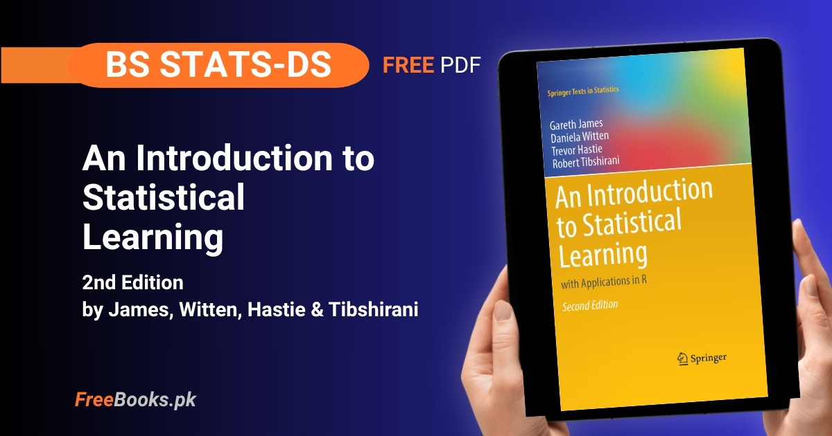
An Introduction to Statistical Learning, Second Edition, by Gareth James, Daniela Witten, Trevor Hastie, and Robert Tibshirani, is the standard first textbook for Statistical Learning and Machine Learning courses in BS Statistics and BS Data Science programs. It covers the full first-course sequence — linear regression, classification, resampling, regularization, tree-based methods, support vector machines, deep learning, survival analysis, unsupervised learning, and multiple testing — building every method on the same bias-variance framework introduced in Chapter 2, so later chapters extend earlier ones instead of starting over.
For BS Data Science and BS Statistics students, this book is built for board-style and semester exam preparation as much as for applied project work: every chapter pairs its theory with an end-of-chapter lab using real data sets — wage data, stock market returns, gene expression, brain-cancer survival times — available in both R (ISLR2 package) and Python (ISLP package) versions, so a student can revise the formulas from the chapter text and then immediately check understanding by reproducing the lab’s results in whichever language their course teaches.
Book Overview
| Course | Statistical Learning / Introduction to Machine Learning |
| Degree Programs | BS Data Science, BS Statistics |
| Level | Undergraduate (final-year core/elective; assumes intro statistics + matrix algebra) |
| Author(s) | Gareth James, Daniela Witten, Trevor Hastie & Robert Tibshirani |
| Publisher | Springer (Springer Texts in Statistics) |
| Edition | 2nd Edition (2021), with the ISLP Python lab edition added in 2023 |
| Structure | 13 chapters, one block below per chapter |
| Labs | End-of-chapter labs in both R (ISLR2 package) and Python (ISLP package) — same theory, same exercises, different lab language |
| Language | English |
| Format | PDF (free download from the authors’ own site) · print/ebook purchasable via Springer or Amazon |
Chapter List
Chapter 1: Introduction
Difficulty: Easy · Key topics: statistical learning, Wage data, Stock Market data, gene expression data, supervised/unsupervised learning, regression vs classification
The authors open by explaining why statistical learning — the set of tools for understanding data that grew out of statistics and merged with machine learning — became essential once cheap sensors, the internet, and genomic sequencing made large, complex data sets routine. Three running examples are introduced and used throughout the rest of the book: the Wage data set (predicting a worker’s wage from age, education, and year, a regression problem), the Smarket Stock Market data (predicting whether the market goes up or down, a classification problem), and the NCI60 gene expression data (grouping cancer cell lines with no response variable at all, an unsupervised problem). The chapter lays out the book’s organization and states plainly that it assumes only an introductory statistics and matrix algebra background, aiming for a less mathematically demanding treatment than the authors’ companion graduate text, The Elements of Statistical Learning.
Key Points:
- Statistical learning = tools for understanding data, spanning both classical statistics and newer machine-learning methods.
Wagedata → a regression example (quantitative output: wage).Smarketdata → a classification example (qualitative output: Up/Down).NCI60data → an unsupervised example (no response variable; the goal is to find structure).- This book is written as a less technical companion to The Elements of Statistical Learning (Hastie, Tibshirani, Friedman).
Memory Tip: Anchor each learning type to its running data set — Wage = regression, Market = classification, NCI60 = unsupervised — and the rest of the book’s examples slot in around these three.
Common Mistake: Students often use “statistical learning” and “machine learning” as if they were two separate subjects taught by two separate courses; the book treats them as one continuous toolbox and expects you to stop drawing that line.
Important Questions:
- What are the book’s three running example data sets, and which learning type does each illustrate? Wage (regression), Smarket (classification), NCI60 (unsupervised learning / no response variable).
- What background does the book assume of its reader? An introductory statistics course and some matrix algebra — it is written to be less mathematically demanding than The Elements of Statistical Learning.
Chapter 2: Statistical Learning
Difficulty: Medium · Key topics: reducible/irreducible error, prediction vs inference, parametric vs non-parametric, bias-variance trade-off, Bayes classifier, K-nearest neighbors
This chapter builds the mathematical framework the rest of the book uses: Y = f(X) + ε, where f is the systematic relationship we want to estimate and ε is random error. It separates two different goals — prediction (just get Y right, f can be a black box) and inference (understand how each predictor X affects Y) — and shows that linear models serve inference well because they are interpretable, while flexible non-linear models like thin-plate splines or random forests chase prediction accuracy at the cost of interpretability. The chapter then derives the expected test MSE as the sum of irreducible error, squared bias, and variance, and uses this bias-variance decomposition to explain why a model that fits the training data perfectly can still predict new data badly (overfitting). It closes with the Bayes classifier as the theoretical gold standard for classification problems and K-nearest neighbors (KNN) as a simple, practical approximation to it.
Key Points:
Y = f(X) + ε— the basic model: a systematic partf(X)plus irreducible random error.- Prediction wants an accurate
f̂; inference wants to understand the relationship between eachXandY. - Parametric methods (e.g. linear regression) assume a functional form and estimate a few parameters; non-parametric methods (e.g. KNN, splines) make no such assumption but need more data.
- Expected test MSE = Var(
f̂(x0)) + [Bias(f̂(x0))]2 + Var(ε) — the bias-variance trade-off. - The Bayes classifier assigns each observation to the class with the highest conditional probability given X — it minimizes test error but requires knowing the true conditional distribution, which is almost never known in practice.
- KNN approximates the Bayes classifier by voting among the K nearest training points; small K → flexible/low bias/high variance, large K → smooth/high bias/low variance.
Memory Tip: Remember the trade-off as a seesaw: pushing flexibility up always lowers bias but raises variance, so the best model sits wherever test error (not training error) is lowest — never judge a model by how well it fits the data it was trained on.
Common Mistake: Choosing the model that gets the lowest training error. A highly flexible model can drive training error toward zero while its test error climbs — the whole point of this chapter is that training error is the wrong thing to minimize.
Important Questions:
- What three quantities make up the expected test MSE, and what happens to each as model flexibility increases? Bias², variance, and irreducible error; bias falls and variance rises as flexibility increases, which is why the sum (test MSE) is typically U-shaped.
- Why is the Bayes classifier only a theoretical benchmark rather than something you can compute directly on real data? It requires the true conditional probability P(Y|X), which is unknown for real data; KNN and other classifiers are practical approximations to it.
Chapter 3: Linear Regression
Difficulty: Medium · Key topics: simple and multiple linear regression, least squares, R², F-statistic, qualitative predictors, interaction effects, collinearity
Linear regression is presented as the foundation that almost every later method either extends or departs from. The chapter develops simple linear regression (one predictor), derives the least-squares estimates of the intercept and slope, and shows how to attach standard errors, confidence intervals, and a hypothesis test (H0: β1 = 0) to the slope coefficient, plus how R² and the residual standard error (RSE) measure fit. It then extends to multiple linear regression with several predictors at once, introduces the F-statistic for testing whether any predictor matters, and works through practical issues: encoding qualitative (categorical) predictors with dummy variables, adding interaction terms when the effect of one predictor depends on another, modelling non-linearity with polynomial terms, and a full catalogue of six potential problems — non-linearity, correlated errors, non-constant variance (heteroscedasticity), outliers, high-leverage points, and collinearity. The chapter ends by comparing linear regression’s parametric assumptions against the fully non-parametric KNN regression from Chapter 2.
Key Points:
- Least squares chooses
β̂0, β̂1to minimize the residual sum of squares (RSS). R²is the fraction of variance inYexplained by the model; theF-statistic tests whether at least one predictor has a non-zero coefficient.- A qualitative predictor with two levels is coded with one 0/1 dummy variable; with more than two levels it needs multiple dummies.
- An interaction term (
X1 × X2) lets the effect of one predictor onYchange with the level of another. - Collinearity (predictors correlated with each other) inflates coefficient standard errors and makes individual effects hard to isolate even when the overall fit is good — check with the Variance Inflation Factor (VIF).
- High-leverage points (unusual
Xvalues) can distort the fitted line far more than outliers (unusualYvalues) do.
Practice Tip: Run cor() (R) or DataFrame.corr() (Python) on your predictors before fitting anything — spotting collinearity before you fit the model saves you from chasing confusing, unstable coefficient estimates afterward.
Common Mistake: Treating a small p-value on an individual predictor as proof that predictor matters in isolation, while ignoring collinearity with another predictor already in the model — the chapter’s Credit data example shows two correlated predictors can each look insignificant together even though the pair is jointly important.
Important Questions:
- What does the F-statistic test that individual t-statistics on each coefficient do not? The F-test checks whether at least one of the predictors is related to the response across the whole model jointly, which matters especially when there are many predictors, since some individual t-tests will look significant by chance alone.
- Why can collinearity be a serious problem even when the model’s overall R² is high? Because it inflates the standard errors of the correlated coefficients, making it hard to tell which of the correlated predictors is actually driving the response, even though the combined fit remains good.
Chapter 4: Classification
Difficulty: Medium · Key topics: logistic regression, linear discriminant analysis (LDA), quadratic discriminant analysis (QDA), naive Bayes, generalized linear models
The chapter opens by showing why ordinary linear regression is a poor fit for a categorical response — predicted values can fall outside [0,1] and the model has no natural way to handle more than two unordered classes — and introduces logistic regression, which models the probability P(Y=1|X) through the logistic function and estimates coefficients by maximum likelihood rather than least squares. It extends logistic regression to multiple predictors and then to more than two classes (multinomial logistic regression), using the Stock Market and Default data sets throughout. The chapter then presents linear discriminant analysis (LDA), which models the predictor distribution within each class as Gaussian and applies Bayes’ theorem to get back to a classification rule, and contrasts it with quadratic discriminant analysis (QDA), which allows each class its own covariance matrix, and naive Bayes, which assumes predictors are independent within each class. It closes with a practical comparison of all these classifiers plus KNN, and a brief look at generalized linear models (Poisson regression) for count data.
Key Points:
- Logistic regression models
p(X) = eᵉ/(1+eᵉ)wherez = β0 + β1X, keeping predicted probabilities between 0 and 1. - Coefficients in logistic regression are estimated by maximum likelihood, not least squares.
- LDA assumes predictors are Gaussian with a shared covariance matrix across classes; QDA relaxes the shared-covariance assumption and fits a separate covariance matrix per class.
- LDA tends to work better with few training observations or well-separated, roughly Gaussian classes; QDA needs more data but can capture non-linear decision boundaries.
- Naive Bayes assumes each predictor is independent within a class — a strong simplification that still works surprisingly well, especially with many predictors.
- No single classifier dominates: the best choice depends on the true decision boundary’s shape and how much training data is available.
Practice Tip: On the Default credit-card data, fit logistic regression, LDA, and QDA side by side and compare their confusion matrices, not just overall accuracy — the book’s own example shows the default rate is low (about 3%), so a model that just predicts “No default” every time looks deceptively accurate.
Common Mistake: Judging a classifier only by overall accuracy on an imbalanced data set. The Default example is specifically built to show that a near-useless classifier can post a high accuracy number while missing almost every true default — always check sensitivity/specificity or the full confusion matrix too.
Important Questions:
- Why does ordinary linear regression fail as a method for binary classification? It can produce fitted probabilities outside the [0,1] range and has no principled way to extend to more than two unordered classes, which is why logistic regression’s bounded logistic function is used instead.
- What is the key structural difference between LDA and QDA? LDA assumes every class shares one common covariance matrix (giving a linear decision boundary); QDA estimates a separate covariance matrix per class (giving a quadratic, more flexible boundary) at the cost of needing more training data.
Chapter 5: Resampling Methods
Difficulty: Medium · Key topics: validation set approach, leave-one-out cross-validation (LOOCV), k-fold cross-validation, bootstrap
This chapter teaches the two core resampling tools used everywhere else in the book to estimate how well a model will really perform. Cross-validation is introduced first through the simple validation-set approach (split once, train on one half, test on the other) and its main weakness — high variance depending on which observations land in which half — motivates leave-one-out cross-validation (LOOCV), which fits the model n times, each time leaving out a single observation, and then k-fold cross-validation, which is the practical compromise used in real work: split the data into k folds (typically 5 or 10), train on k-1 folds and validate on the one left out, and average the k resulting error estimates. The chapter works out the bias-variance trade-off of this choice: LOOCV has lower bias but higher variance than k-fold CV, so k = 5 or 10 is the commonly recommended sweet spot. The second half of the chapter introduces the bootstrap, a general resampling technique for quantifying the uncertainty (standard errors, confidence intervals) of almost any statistic by repeatedly resampling the observed data with replacement.
Key Points:
- The validation-set approach can give highly variable test-error estimates because the result depends heavily on which observations happened to land in the validation half.
- LOOCV fits the model
ntimes (leaving out one observation each time) — low bias, but can be computationally expensive and has relatively high variance. k-fold CV (commonlyk=5ork=10) trades a small increase in bias for a useful reduction in variance compared to LOOCV, and is far cheaper to compute.- For least-squares linear/polynomial regression, LOOCV has a shortcut formula and does not actually require refitting the model
nseparate times. - The bootstrap estimates the variability of a statistic (e.g. a regression coefficient) by resampling the observed data with replacement, without relying on any formula or distributional assumption.
Practice Tip: Always set a random seed (set.seed() in R, np.random.seed()/a random_state in Python) before cross-validation or bootstrapping so a reported error estimate can actually be reproduced on a re-run.
Common Mistake: Running cross-validation on data that was already used to select features or tune the model (e.g. choosing which predictors to include based on the whole data set, then cross-validating the final model) — this leaks information and produces an overly optimistic error estimate; CV must wrap the entire modelling process, not just the final fit.
Important Questions:
- Why is k-fold cross-validation (k=5 or 10) usually preferred over LOOCV in practice? LOOCV has lower bias but higher variance and is far more computationally expensive for most models; k-fold CV accepts a little more bias in exchange for lower variance and dramatically less computation.
- What problem does the bootstrap solve that cross-validation does not? The bootstrap quantifies the uncertainty (e.g. standard error or confidence interval) of a statistic or estimator itself, rather than estimating a model’s prediction error on new data, which is what cross-validation is for.
Chapter 6: Linear Model Selection and Regularization
Difficulty: Medium-Hard · Key topics: best subset selection, forward/backward stepwise selection, ridge regression, the lasso, principal components regression (PCR), partial least squares (PLS)
With many available predictors, this chapter asks how to choose a smaller, better-performing model than the one that simply includes every predictor. It first covers subset-selection methods — best subset selection (try every possible combination of predictors, infeasible beyond a few dozen predictors), and the cheaper forward and backward stepwise selection, which add or remove one predictor at a time — alongside criteria for comparing models of different sizes (adjusted R², Akaike Information Criterion (AIC), Bayesian Information Criterion (BIC), and cross-validation). It then turns to shrinkage methods that keep every predictor but constrain their coefficients: ridge regression adds an L2 penalty that shrinks coefficients toward zero without ever setting them exactly to zero, while the lasso’s L1 penalty can shrink some coefficients all the way to zero, which performs variable selection automatically and produces a sparser, more interpretable model. The chapter closes with dimension-reduction methods — principal components regression (PCR), which regresses on a small number of principal components of the predictors, and partial least squares (PLS), which builds those components using the response variable as well — and discusses the special challenges of high-dimensional data (p > n), where the usual R² and p-value interpretations break down.
Key Points:
- Best subset selection searches all
2^ppossible predictor combinations — exact but computationally infeasible oncepis more than a few dozen. - Forward stepwise selection starts empty and adds the best predictor at each step; backward stepwise starts full and removes the least useful predictor — both are greedy and not guaranteed to find the true best model.
- Ridge regression’s penalty is
λΣβj²(L2) — shrinks all coefficients toward zero but keeps them all in the model. - The lasso’s penalty is
λΣ|βj|(L1) — can force some coefficients to exactly zero, giving automatic variable selection. - The tuning parameter
λin ridge/lasso is chosen by cross-validation;λ=0recovers ordinary least squares. - PCR reduces dimensionality using the predictors alone (unsupervised); PLS does the same but uses the response to guide which directions matter most (supervised).
Practice Tip: Standardize (scale) every predictor before fitting ridge or lasso — both penalties are scale-sensitive, so a predictor measured in different units can be penalized unfairly more or less than the others if you skip this step.
Common Mistake: Assuming the lasso is always better than ridge because it also does variable selection. When most predictors genuinely contribute a little (no truly sparse true model), ridge regression typically gives better prediction accuracy than the lasso — which method wins depends on the true underlying model, not on a general rule.
Important Questions:
- What is the key practical difference between ridge regression and the lasso? Ridge regression’s L2 penalty shrinks all coefficients toward zero but never to exactly zero, so it keeps every predictor; the lasso’s L1 penalty can shrink some coefficients to exactly zero, performing variable selection and producing a sparser, more interpretable model.
- Why do best subset and stepwise selection become impractical with many predictors, and what replaces them? Best subset selection requires fitting
2^pmodels, which is computationally infeasible beyond a few dozen predictors; forward/backward stepwise selection or the shrinkage methods (ridge, lasso) are used instead for largerp.
Chapter 7: Moving Beyond Linearity
Difficulty: Medium · Key topics: polynomial regression, step functions, regression splines, smoothing splines, local regression, generalized additive models (GAMs)
This chapter relaxes the strict linearity assumption of earlier chapters one step at a time. Polynomial regression adds powers of a predictor to capture curvature; step functions instead cut the predictor’s range into bins and fit a separate constant in each. Regression splines combine the two ideas by fitting piecewise polynomials that are forced to join smoothly at a set of knots, and the chapter explains how more knots increase flexibility (and variance) the same way higher polynomial degree does. Smoothing splines take the opposite route: start from a function that interpolates every point exactly, then penalize roughness directly so that a single tuning parameter (chosen by cross-validation) controls the flexibility, without the user needing to choose knot locations by hand. Local regression fits a separate weighted regression at every target point using only its nearby neighbors. The chapter closes by combining all of these one-predictor tools into generalized additive models (GAMs), which fit a separate smooth function to each predictor and add the results together, keeping the interpretability of “one effect per predictor” while allowing each effect to be non-linear.
Key Points:
- Polynomial regression fits
y = β0 + β1x + β2x² + ... + βdx^d— the degreedcontrols flexibility. - A regression spline is a piecewise polynomial constrained to be continuous (and usually smooth in its first and second derivatives) at a chosen set of knots.
- A smoothing spline avoids choosing knot locations: it minimizes RSS plus a roughness penalty
λ∫f''(x)²dx, withλset by cross-validation. - Local regression weights nearby points more heavily when fitting the value at each target point, controlled by a “span” parameter.
- GAMs extend linear models by replacing each linear term with a smooth function, e.g.
y = β0 + f1(x1) + f2(x2) + ... + ε, keeping per-predictor interpretability.
Practice Tip: Plot each fitted non-linear function against its predictor before trusting it — a spline or smoothing-spline fit with too many knots or too small a λ will visibly wiggle to chase noise, which is easy to catch by eye but easy to miss by looking at R² alone.
Common Mistake: Picking the polynomial degree or number of knots by eye on the training data instead of by cross-validation. Both regression splines and polynomial terms will always fit the training data at least as well with more flexibility, so an un-cross-validated choice systematically overfits.
Important Questions:
- What problem do regression splines solve that plain polynomial regression does not? A single high-degree polynomial applies the same global curvature everywhere, which can produce wild behavior near the boundaries; regression splines fit separate, lower-degree polynomials in different regions joined smoothly at knots, giving more local control over the fit.
- How does a generalized additive model (GAM) stay interpretable while still being non-linear? It fits one smooth function per predictor and adds the effects together, so you can still look at and interpret the individual effect of each predictor, unlike a fully joint non-linear model where effects are tangled together.
Chapter 8: Tree-Based Methods
Difficulty: Medium · Key topics: decision trees, bagging, random forests, boosting, Bayesian additive regression trees (BART)
The chapter starts with a single decision tree, built by recursive binary splitting of the predictor space to minimize RSS (regression trees) or a measure like the Gini index or entropy (classification trees), followed by pruning back a large tree using cost-complexity pruning to avoid overfitting. A single tree is easy to interpret but has high variance — a small change in the training data can produce a very different tree — which motivates the rest of the chapter’s ensemble methods. Bagging (bootstrap aggregation) averages many trees, each grown on a different bootstrap sample of the data, to reduce variance. Random forests go one step further: at each split, only a random subset of predictors is considered, which decorrelates the trees (otherwise a single dominant predictor would make every bagged tree look similar) and typically improves prediction further. Boosting grows trees sequentially, where each new tree is fit to the residuals left over by the current ensemble, slowly improving the fit using a learning-rate parameter to control how much each tree contributes. The chapter closes with Bayesian additive regression trees (BART), which combines ideas from bagging and boosting within a Bayesian framework.
Key Points:
- A regression tree splits the predictor space to minimize RSS; a classification tree splits to minimize the Gini index or cross-entropy.
- Cost-complexity pruning grows a large tree first, then prunes it back using a penalty on tree size, with the penalty strength chosen by cross-validation.
- Bagging averages trees grown on bootstrap samples of the training data, which reduces variance without increasing bias much.
- Random forests decorrelate bagged trees by considering only
m ≈ √prandomly chosen predictors at each split (for classification); this usually outperforms plain bagging. - Boosting fits trees sequentially to the current residuals, controlled by a learning rate (shrinkage parameter) — unlike bagging/random forests, the trees are not independent.
- Variable importance measures (e.g. total decrease in RSS/Gini index from splits on a predictor) let tree ensembles recover some of the interpretability that a single tree has and an ensemble otherwise loses.
Practice Tip: Tune a random forest’s mtry (number of predictors sampled per split) and a boosted model’s learning rate + number of trees by cross-validation rather than defaults — the book’s own examples on the Boston and Carseats data sets show both parameters materially change test error.
Common Mistake: Using more boosting iterations (trees) always helps, so cranking the number up is “safer.” Unlike random forests, boosting CAN overfit if you add too many trees or set the learning rate too high — the number of trees is a tuning parameter to select by cross-validation, not a value to maximize.
Important Questions:
- How do random forests improve on plain bagging of decision trees? By restricting each split to a random subset of the available predictors, random forests decorrelate the individual trees (bagging alone can produce very similar trees when one predictor dominates), which further reduces the variance of the averaged prediction.
- What is the fundamental difference between how bagging/random forests and boosting build their ensemble of trees? Bagging and random forests grow trees independently and in parallel on bootstrap samples and then average them; boosting grows trees sequentially, with each new tree fit to the residual error left by the trees already in the ensemble.
Chapter 9: Support Vector Machines
Difficulty: Hard · Key topics: maximal margin classifier, support vector classifier, support vector machine, kernels, multiclass extensions
The chapter builds support vector machines (SVMs) in three stages of increasing generality. The maximal margin classifier finds the hyperplane that separates two perfectly linearly separable classes while maximizing the margin (the distance to the nearest point of either class) — elegant, but it only exists when the classes really are perfectly separable and is highly sensitive to individual observations near the boundary. The support vector classifier relaxes this by allowing a “soft margin”: some observations are permitted to sit on the wrong side of the margin or even the hyperplane, controlled by a budget parameter C, which trades bias for variance much like other tuning parameters in the book. The support vector machine itself extends the support vector classifier to non-linear decision boundaries using the kernel trick — rather than literally expanding the feature space, a kernel function (polynomial, radial/RBF) computes the inner products that a classifier needs as if the expansion had happened, at much lower computational cost. The chapter closes by extending binary SVMs to more than two classes via one-versus-one and one-versus-all approaches, and relates SVMs to logistic regression, noting the two methods often give similar results when classes are not well separated.
Key Points:
- The maximal margin classifier exists only for perfectly, linearly separable classes and maximizes the margin between the hyperplane and the nearest training points (the support vectors).
- The support vector classifier introduces a cost parameter
Cthat controls how many violations of the margin are tolerated — smallC→ narrow margin, low bias, high variance; largeC→ wide margin, higher bias, lower variance. - The kernel trick lets an SVM fit non-linear boundaries by implicitly computing inner products in an enlarged feature space, without ever forming that expanded space explicitly.
- Common kernels: linear (≈ support vector classifier), polynomial (degree
d), and radial/RBF (controlled byγ), each giving a different boundary shape. - Only the support vectors (points on or inside the margin) determine the decision boundary — moving any other point does not change the fitted classifier at all.
- For more than two classes, SVMs are usually extended via one-versus-one (fit a classifier for every pair of classes) or one-versus-all.
Practice Tip: Always tune both the cost parameter C and any kernel-specific parameter (e.g. γ for the radial kernel) together via cross-validation on a grid — tuning one while leaving the other at its default commonly used in the lab’s tune() function gives a misleadingly poor picture of what the kernel can actually do.
Common Mistake: Assuming a radial/non-linear kernel will always outperform a linear SVM. When the true boundary really is close to linear, a radial kernel’s extra flexibility adds variance without adding useful bias reduction — the book’s own simulated examples are built specifically to show a linear SVM beating a radial one when the true separation is linear.
Important Questions:
- What problem does the support vector classifier solve that the maximal margin classifier cannot? The maximal margin classifier is only defined when the two classes are perfectly linearly separable; the support vector classifier introduces a soft margin (controlled by cost parameter
C) that tolerates some misclassified or margin-violating points, so it still works on realistic, non-separable data. - What does the “kernel trick” actually avoid computing? It avoids ever explicitly constructing the enlarged (possibly very high- or infinite-dimensional) feature space; the kernel function computes the inner products the SVM needs directly from the original features, which is what makes non-linear SVMs computationally practical.
Chapter 10: Deep Learning
Difficulty: Hard · Key topics: single and multilayer neural networks, convolutional neural networks (CNNs), recurrent neural networks (RNNs), backpropagation, dropout, double descent
New to the 2nd edition, this chapter introduces neural networks from the ground up using the same regression/classification framing as the rest of the book. It starts with a single-layer network (essentially a non-linear generalization of linear/logistic regression with one hidden layer of “activation units”), then stacks multiple hidden layers into a multilayer network and shows this is what is usually meant by “deep learning.” Convolutional neural networks (CNNs) are introduced for image data, built from convolution layers (that detect local patterns such as edges using small filters) and pooling layers (that downsample and build translation-invariance), illustrated on a digit- and image-classification example. Recurrent neural networks (RNNs) are introduced for sequential data — document classification and time-series/language-model examples are worked through — explaining how a hidden state carries information from earlier elements of a sequence to later ones. The chapter covers how these networks are actually fit via backpropagation and stochastic gradient descent, and how overfitting in a model with far more parameters than observations is controlled using dropout, weight penalties (ridge/lasso-style), and early stopping. It closes with the double-descent phenomenon, where test error can fall again (after first rising, as classical bias-variance theory predicts) once a model becomes flexible enough to interpolate the training data, which complicates the simple “more flexible = more overfit” intuition from Chapter 2 for very large networks.
Key Points:
- A single-layer neural network computes hidden units as non-linear transformations (activation functions, e.g. ReLU or sigmoid) of weighted sums of the inputs, then combines those hidden units linearly for the output.
- A deep network stacks multiple hidden layers; each additional layer lets the network represent increasingly abstract combinations of the previous layer’s features.
- CNNs use convolution layers (local filters shared across the image) and pooling layers (downsampling) — built for image data where nearby pixels are related.
- RNNs maintain a hidden state updated at every step of a sequence, which is what lets them handle inputs of varying length like text or time series.
- Networks are fit by minimizing a loss function via (stochastic) gradient descent, with gradients computed efficiently by backpropagation.
- Dropout (randomly zeroing out a fraction of hidden units during training) is a regularization technique specific to neural networks, alongside more familiar weight penalties.
- Double descent: as model flexibility keeps increasing past the point of perfectly fitting (interpolating) the training data, test error can decrease again, which does not fit the simple U-shaped bias-variance picture from Chapter 2.
Practice Tip: Work through the chapter’s own image-classification (CNN) and document-classification (RNN) lab examples end to end rather than reading the architecture diagrams alone — the training-curve plots in the lab are what actually make dropout and early stopping’s effect on overfitting visible.
Common Mistake: Assuming any neural network automatically beats the simpler models from earlier chapters. The chapter’s own Hitters and other tabular-data comparisons show a well-tuned lasso or random forest often matches or beats a neural network on small, structured (non-image, non-text) data sets — deep learning’s advantage shows up mainly on image, text, and other unstructured data with lots of observations.
Important Questions:
- What structural feature of CNNs makes them well suited to image data specifically? Convolution layers apply small filters that are shared across the whole image to detect local patterns (like edges) regardless of where they occur, and pooling layers then downsample for translation-invariance — both exploit the fact that nearby pixels in an image are related.
- What is the double-descent phenomenon, and why does it complicate the Chapter 2 bias-variance picture? As model flexibility increases far enough to exactly interpolate the training data, test error, after first rising as classical theory predicts, can fall again — a second descent that the simple “more flexible always eventually overfits more” intuition from Chapter 2 does not predict.
Chapter 11: Survival Analysis and Censored Data
Difficulty: Medium-Hard · Key topics: censoring, Kaplan-Meier estimator, log-rank test, hazard function, Cox proportional hazards model
Also new to the 2nd edition, this chapter handles response variables that are “time until an event” (death, equipment failure, customer churn) where some observations are censored — the event had not yet happened when the data was collected, so the exact survival time is unknown, only a lower bound on it. The Kaplan-Meier estimator is introduced as the standard non-parametric way to estimate the survival curve (the probability of surviving past time t) from censored data, worked through on the book’s brain-cancer and publication-time examples. The log-rank test is then used to compare survival curves between two or more groups (e.g. by sex or treatment) without assuming any particular distributional form. The chapter moves to regression for survival data via the hazard function (the instantaneous risk of the event at time t, given survival up to t) and builds up to the Cox proportional hazards model, a semi-parametric regression model that estimates how predictors multiply the baseline hazard without needing to specify that baseline hazard’s exact shape. It closes by connecting shrinkage methods (ridge, lasso) from Chapter 6 to the Cox model for survival data with many predictors.
Key Points:
- Censoring means the exact event time is unknown for some observations — only that it occurred after a known point — and simply dropping censored observations biases the analysis.
- The Kaplan-Meier estimator gives a non-parametric estimate of the survival function
S(t) = P(T > t)that correctly accounts for censoring. - The log-rank test compares two or more Kaplan-Meier curves to test whether survival differs across groups, without assuming a parametric survival distribution.
- The hazard function
h(t)is the instantaneous risk of the event at timet, conditional on survival up tot— it underlies every survival regression model in the chapter. - The Cox proportional hazards model assumes predictors act multiplicatively on a baseline hazard that is never explicitly estimated, which is why it is called semi-parametric.
- “Proportional hazards” means the ratio of hazards between any two individuals is assumed constant over time — a key assumption to check, not just assume.
Memory Tip: Keep Kaplan-Meier, log-rank, and Cox straight by what each answers: Kaplan-Meier describes one group’s survival curve, the log-rank test compares curves between groups, and the Cox model adds predictors to explain differences in hazard quantitatively.
Common Mistake: Treating censored observations as if the event simply never happened (coding them as “survived,” or dropping them from the data set). Both choices bias the survival estimate — censored observations must be handled by the Kaplan-Meier/Cox machinery specifically built for partial information, not discarded or recoded.
Important Questions:
- What is censoring, and why can’t censored observations simply be removed from a survival analysis? Censoring means the true event time is unknown for an observation, only that it is at least as large as the observed (censored) time; removing these observations discards real partial information and biases the survival estimate, typically making survival look shorter than it really is.
- What does the Cox proportional hazards model assume about how predictors affect risk over time? It assumes proportional hazards — that the ratio of the hazard functions for any two sets of predictor values stays constant over time, even though the baseline hazard itself is never directly estimated.
Chapter 12: Unsupervised Learning
Difficulty: Medium · Key topics: principal component analysis (PCA), matrix completion, k-means clustering, hierarchical clustering
Unsupervised learning drops the response variable entirely and asks what structure the predictors alone reveal. Principal component analysis (PCA) is presented first as both a visualization tool and a dimension-reduction technique: it finds the directions (principal components) along which the data varies the most, in order, and the chapter works through how much of the total variance each component explains and how to decide how many components to keep. A section on missing values and matrix completion extends PCA-style ideas to filling in gaps in a data matrix (e.g. a user-ratings matrix), connecting to the kind of problem behind recommender systems. The chapter then turns to clustering: k-means clustering partitions observations into a pre-chosen number of K clusters by iteratively assigning each point to its nearest cluster centroid and recomputing centroids, while hierarchical clustering instead builds a full tree (dendrogram) of nested clusters without committing to a number of clusters up front, using a choice of linkage (complete, average, single, centroid) to decide how to measure distance between clusters. The chapter closes with practical issues common to all clustering methods: whether and how to scale variables first, sensitivity to outliers, and the fact that there is no universally “correct” number of clusters to validate against.
Key Points:
- PCA finds a sequence of orthogonal directions (principal components) that successively capture the most variance in the data, useful for both visualization and dimension reduction.
- The proportion of variance explained (PVE) by each component, often shown in a scree plot, guides how many components to retain.
- K-means requires choosing
Kin advance and can converge to different results depending on the random starting centroids, so it is usually run multiple times from different starts. - Hierarchical clustering produces a dendrogram that can be cut at any height to yield any number of clusters, without re-running the algorithm.
- The choice of linkage (complete, average, single, centroid) in hierarchical clustering materially changes the resulting cluster shapes.
- Unlike supervised learning, there is no response variable to validate against, so cluster quality is judged by domain knowledge and stability, not by a test-error number.
Practice Tip: Always scale (standardize) variables before k-means or PCA unless every variable is already on a comparable scale — a variable measured in larger units will otherwise dominate the distance calculation or the first principal component purely because of its scale, not because it is actually more important.
Common Mistake: Treating the output of k-means or hierarchical clustering as “the” correct grouping. Because there is no ground truth in unsupervised learning, running the same algorithm with a different K, a different linkage, or different scaling can produce a genuinely different, equally defensible clustering — results should always be checked for stability, not reported as the single right answer.
Important Questions:
- What is the key practical difference between k-means and hierarchical clustering? K-means requires the number of clusters
Kto be chosen in advance and partitions the data directly into that many groups; hierarchical clustering builds a full nested tree (dendrogram) first and lets you choose the number of clusters afterward by deciding where to cut it. - Why can’t PCA or clustering results be validated the way a regression or classification model is, using a test set? There is no response variable in unsupervised learning, so there is no “correct answer” to measure prediction error against — results are instead judged by domain knowledge, interpretability, and stability across resampled data or algorithm settings.
Chapter 13: Multiple Testing
Difficulty: Medium · Key topics: family-wise error rate (FWER), Bonferroni and Holm corrections, false discovery rate (FDR), Benjamini-Hochberg procedure, resampling-based p-values
The book’s final chapter, also new to the 2nd edition, tackles what goes wrong when many hypothesis tests are run at once — a routine situation in genomics, A/B testing, and any analysis that screens many predictors. It starts by reviewing a single hypothesis test’s Type I/Type II error framework, then shows that testing m hypotheses at a 0.05 significance level each lets the family-wise error rate (FWER, the probability of at least one false positive across all m tests) grow quickly toward 1 as m increases, using the formula FWER = 1-(1-α)^m for independent tests. The Bonferroni correction (divide α by m) and the slightly less conservative Holm’s step-down procedure are presented as ways to control FWER, both of which become very conservative (low power to detect real effects) as m grows large. The chapter then introduces the false discovery rate (FDR) as a more practical alternative in large-scale settings like genomics: instead of trying to avoid any false positive at all, FDR control accepts a fixed proportion of false positives among all rejected hypotheses, implemented via the Benjamini-Hochberg procedure. It closes with a resampling-based approach (using permutation) to compute p-values and control these error rates without relying on strict distributional assumptions, illustrated on gene-expression data.
Key Points:
- Family-wise error rate (FWER) is the probability of making at least one false rejection across all
mtests — it grows toward 1 quickly asmincreases if each test is run at the usual 0.05 level. - The Bonferroni correction controls FWER by testing each hypothesis at level
α/m— simple but very conservative for largem. - Holm’s step-down procedure also controls FWER but is uniformly more powerful than Bonferroni, since it adjusts the threshold sequentially rather than dividing by a fixed
m. - The false discovery rate (FDR) is the expected proportion of false positives among all rejected hypotheses — a more forgiving and more useful standard than FWER when testing thousands of hypotheses, as in genomics.
- The Benjamini-Hochberg procedure controls FDR at a target level by ranking p-values and finding the largest rank whose p-value is below a sliding threshold.
- When the true null distribution of a test statistic is unclear or test statistics are correlated, a permutation-based (resampling) approach can compute valid p-values and error-rate estimates directly from the data.
Memory Tip: FWER asks “did I make even ONE mistake across everything?” (strict); FDR asks “what fraction of my positive findings are mistakes?” (forgiving) — use FWER control (Bonferroni/Holm) when a single false positive is costly, and FDR control (Benjamini-Hochberg) when you expect and can tolerate some false positives among many discoveries, which is the usual genomics/large-scale-screening situation.
Common Mistake: Running dozens or hundreds of tests (e.g. testing every gene, every predictor, every subgroup) and reporting the handful that happen to come back significant at the uncorrected 0.05 level. This is exactly the scenario this chapter exists to warn against — without a FWER or FDR correction, some “significant” results are expected purely by chance even if nothing real is going on.
Important Questions:
- What is the practical difference between controlling FWER and controlling FDR? FWER control (Bonferroni, Holm) tries to guarantee no false positives at all across every test, which becomes very conservative as the number of tests grows; FDR control (Benjamini-Hochberg) instead bounds the expected proportion of false positives among the rejected hypotheses, allowing more true discoveries at the cost of tolerating some false ones — the standard choice in large-scale settings like genomics.
- Why does running many hypothesis tests at the usual α=0.05 level per test become a problem even if every null hypothesis happens to be true? Because the family-wise error rate (the chance of at least one false rejection) rises toward 1 as the number of independent tests
mgrows, following FWER = 1-(1-0.05)^m — so some tests will look “significant” purely by chance even when nothing real is happening.
Download An Introduction to Statistical Learning PDF (Free)
Click below to open the book’s official site — it links straight to the free PDF for both the R and Python lab editions, directly from the authors.
↓ Download PDFHow to Study This Book
Read Chapters 1-2 first even if you already know basic statistics — the bias-variance trade-off and the prediction-vs-inference distinction introduced here are the vocabulary every later chapter assumes you already have. Chapter 3 (Linear Regression) and Chapter 4 (Classification) form the core first course: most BS Statistics and BS Data Science syllabi in Pakistan map a semester’s “Applied Regression” or “Statistical Learning I” course almost directly onto these two chapters plus Chapter 5 (Resampling Methods), which you need before Chapter 6 makes any sense, since every shrinkage method in Chapter 6 depends on cross-validation from Chapter 5 to choose its tuning parameter.
Chapters 6-9 (Regularization, Splines/GAMs, Trees, SVMs) are best read in order, since each introduces one more layer of model flexibility building on the bias-variance ideas from Chapter 2 — do not skip Chapter 6 to jump straight to Chapter 8’s trees, because the idea of a tuning parameter selected by cross-validation, first fully worked out for ridge/lasso, is reused without re-explanation for every tree ensemble and SVM parameter afterward.
Chapters 10-13 (Deep Learning, Survival Analysis, Unsupervised Learning, Multiple Testing) are largely independent of each other and can be read in any order once Chapters 1-9 are solid — pick based on your course: a machine-learning-heavy BS Data Science course usually prioritizes Chapter 10 (Deep Learning) and Chapter 12 (Unsupervised Learning/PCA/clustering); a BS Statistics course with a biostatistics or actuarial leaning should prioritize Chapter 11 (Survival Analysis); and anyone doing an undergraduate research project involving gene expression data, A/B testing, or screening many predictors needs Chapter 13 (Multiple Testing) specifically.
If your course is R-based, work through the end-of-chapter labs using the ISLR2 R package; if it is Python-based, use the identical labs from the ISLP Python package instead — the theory and exercises in every chapter are the same either way, only the lab code differs, so do not re-read a chapter just because your course switched lab language.
Do the end-of-chapter “Conceptual” exercises before the “Applied” (coding) ones in each chapter — the conceptual exercises catch gaps in understanding the formulas (like deriving the bias-variance decomposition yourself for Chapter 2, or working out why ridge regression’s solution always exists even when ordinary least squares does not) before you move to fitting real models in R or Python.
This book does not cover: experimental design (how to collect data in the first place), Bayesian statistics beyond the brief Bayes-classifier framing in Chapter 2 and BART in Chapter 8, or natural-language-specific deep learning architectures like transformers (RNNs in Chapter 10 predate and are distinct from transformer-based models) — students needing those topics should treat this book as the prerequisite, not the complete syllabus.
Used In These Programs
This book is used for the Statistical Learning / Machine Learning course in: BS Data Science · BS Statistics. Browse all Statistical Learning books, all Machine Learning books, or all Statistics books.
Who Should Read This
This book is written for BS Data Science and BS Statistics students taking their first Statistical Learning or Machine Learning course, and it assumes only an introductory statistics course and basic matrix algebra — no prior exposure to machine learning is needed. It is not a pure programming book: the R and Python labs exist to demonstrate the statistics, so a student looking only to learn R or Python from scratch should start with a dedicated programming text like Think Python first and come back once comfortable with basic syntax. It is also not the right starting point for a graduate-level theoretical treatment of these same methods — students who finish this book and want the full mathematical derivations behind it should move on to the authors’ companion graduate text, The Elements of Statistical Learning. Within Pakistani university programs, it is commonly the required or recommended text for courses named “Statistical Learning,” “Introduction to Machine Learning,” or “Applied Predictive Modeling” in the final two years of a BS Statistics or BS Data Science degree, and its Chapter 2 bias-variance framework is frequently referenced again in later data-mining or applied-ML electives.
Applicable Universities
This book is useful for students at Pakistani universities offering BS Data Science and BS Statistics, including Punjab University, Virtual University, COMSATS, FAST, LUMS, NUST, and other HEC-recognized institutions running a Statistical Learning or Introduction to Machine Learning course as part of these degrees.
FAQs
Is An Introduction to Statistical Learning free?
Yes, the PDF is free to download directly from the authors’ own official site, statlearning.com. There is no Creative Commons or open licence on the text itself — the copyright stays with Springer Nature — but the authors make the PDF freely downloadable alongside the paid print and ebook editions sold through Springer and Amazon.
Which edition is this, and is it R or Python?
This page covers the 2nd Edition (2021). The 2nd Edition exists in two lab versions covering identical theory and chapters: the original R labs (ISLR, using the ISLR2 R package) and, since 2023, a Python lab edition (ISLP, using the ISLP Python package, with Jonathan Taylor joining as a contributing author for the Python translation). Pick whichever lab language your course uses — the chapter text is the same either way.
How many chapters does it have, and what’s new in the 2nd Edition?
13 chapters. Three are entirely new compared to the 1st Edition (2013): Chapter 10 (Deep Learning), Chapter 11 (Survival Analysis and Censored Data), and Chapter 13 (Multiple Testing). If you find an older PDF online that stops at 10 or 11 chapters, it is the 1st Edition and is missing this newer material.
Is it good for complete beginners to machine learning?
Yes for the statistics and machine-learning content — it assumes no prior ML background and builds every method from the bias-variance framework in Chapter 2 onward. It does assume you already know basic statistics (distributions, hypothesis tests) and matrix algebra, and it is not a from-scratch R or Python programming tutorial, so complete programming beginners should learn basic R or Python syntax first.
Does it cover deep learning and neural networks?
Yes — Chapter 10, new in the 2nd Edition, covers single and multilayer neural networks, convolutional neural networks (CNNs) for images, and recurrent neural networks (RNNs) for sequential data, including how they are fit (backpropagation, dropout) and the double-descent phenomenon. It is an introduction, not a dedicated deep-learning text, and does not cover transformer architectures.
Does it include solved exercises and real data sets?
Yes. Every chapter ends with Conceptual exercises (work by hand/derive) and Applied exercises (fit models in R or Python) built around real data sets used throughout the book — Wage, Smarket (stock market), Default, Credit, Boston, Hitters, NCI60 gene expression, and BrainCancer survival data among others — plus a full worked lab per chapter that demonstrates the chapter’s methods step by step.
Related Books
- Think Python PDF Download – Allen B. Downey (3rd Edition)
- Problem Solving with Algorithms and Data Structures using Python – Free Book
- Calculus Volume 1 PDF Download – Strang & Herman (OpenStax)
- Discrete Mathematics: An Open Introduction PDF Download – Oscar Levin (4th Edition)
An Introduction to Statistical Learning takes a BS Data Science or BS Statistics student from the basic bias-variance trade-off all the way through regularization, tree ensembles, support vector machines, deep learning, survival analysis, and multiple testing, using the same running real-world data sets at every step and matching R and Python labs so either track of a course can follow along. Browse more Statistics books on Freebooks.pk.
An Introduction to Statistical Learning with Applications in R/Python, 2nd Edition, by Gareth James, Daniela Witten, Trevor Hastie, and Robert Tibshirani. Published by Springer (Springer Texts in Statistics), © Springer Nature 2021. The PDF is made freely downloadable by the authors at the book’s official site; all rights otherwise remain with the publisher. Official source: statlearning.com.
© Copyright Policy
Freebooks.pk is an educational resource for students in Pakistan. Textbooks and other books belong to their respective boards, authors and publishers, and all rights remain with them. If you are the copyright holder of any material on this page and want it changed or removed, please contact us or file a request under our DMCA policy. We review every request and remove reported content promptly.