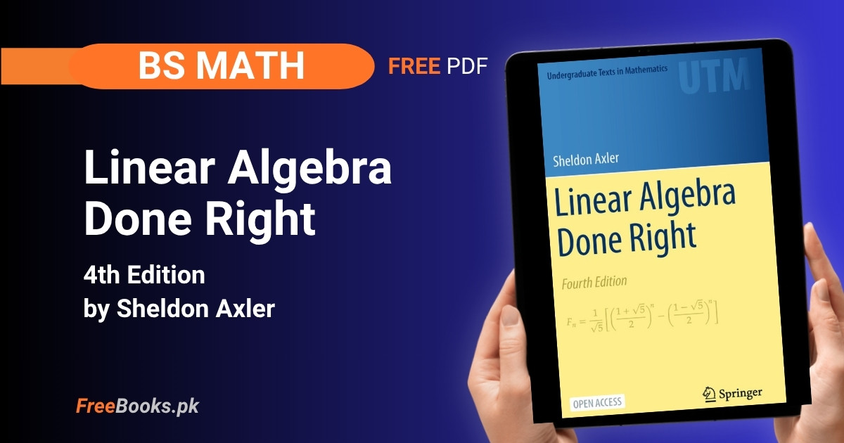
Axler’s Linear Algebra Done Right is the book many mathematics departments choose for a second course in linear algebra, and the fourth edition is free on the author’s official page. Students in BS Mathematics usually meet it after a first course on matrices and systems. It starts again from the definition of a vector space and builds the theory of linear maps and operators on finite-dimensional spaces, with every result proved.
The path is deliberate. Eigenvalues are shown to exist without determinants, and determinants appear only in the last chapter, defined through alternating multilinear forms. In between come inner product spaces, the spectral theorem, the singular value decomposition, and Jordan form. Readers should be comfortable with proofs and ready to work through the exercises on paper; it is a study book for mathematics majors, not a collection of computational recipes.
Book Overview
| Course | Linear Algebra (second course, proof-based) |
| Degree Programs | BS Mathematics |
| Level | Undergraduate — mathematical maturity expected; no prior linear algebra assumed, but the pace and proofs suit a second exposure |
| Edition | Fourth edition — PDF dated 16 August 2026 on the title page (copyright 2024); the author’s page lists it as the most recent edition |
| Author | Sheldon Axler, San Francisco State University |
| Structure | 9 chapters (Vector Spaces; Finite-Dimensional Vector Spaces; Linear Maps; Polynomials; Eigenvalues and Eigenvectors; Inner Product Spaces; Operators on Inner Product Spaces; Operators on Complex Vector Spaces; Multilinear Algebra and Determinants), 35 exercise sets, no appendices |
| Exercises | Roughly 730 proof-oriented exercises across the book (our count); the PDF has no solutions section |
| Language | English (free Chinese, Farsi and Hebrew translations are linked from the official page) |
| License | Creative Commons Attribution-NonCommercial 4.0 International (CC BY-NC 4.0), as printed in the book — Model: Link-only |
| Format | Free PDF, plus a free Kindle version and an accessible HTML version, all linked from the official page; print edition published by Springer |
Chapter List
Chapter 1: Vector Spaces
Difficulty: Medium · Key topics: complex numbers, F^n, vector space axioms, subspaces, sums, direct sums
Starts by building the complex numbers as ordered pairs a + bi, then lifts the familiar plane and 3-space to R^n and C^n, where the letter F stands for either field of scalars. From there the book abstracts to the full definition of a vector space, with examples such as sequences and functions, and proves the first consequences: a unique zero, unique inverses, and 0v = 0. The last section covers subspaces, sums of subspaces, and direct sums, which are used again in almost every later chapter.
Key Points:
- F denotes R or C throughout the book; most results are proved for both at once
- A vector space is a set with addition and scalar multiplication obeying the usual algebraic laws (commutativity, associativity, identity, inverses, distributivity)
- The additive identity and additive inverses are unique, 0v = 0, and (-1)v = -v
- A subset U of V is a subspace if it contains 0 and is closed under addition and scalar multiplication
- U1 + … + Un is the smallest subspace containing all of U1, …, Un
- A sum is a direct sum when the only way to write 0 as a sum of vectors from the pieces is with every vector equal to 0; for two subspaces this means U ∩ W = {0}
Memory Tip: Think of a sum of subspaces as a union that has been “completed” so that addition works, and a direct sum as a union with no overlap except the unavoidable shared zero vector.
Common Mistake: Assuming the union of two subspaces is a subspace. It usually is not; the sum U + W is the object that stays closed under addition.
Important Questions:
- What must you check to show that a subset U of a vector space V is a subspace? That U contains the zero vector, is closed under addition, and is closed under scalar multiplication.
- When is the sum of two subspaces U and W a direct sum? Exactly when U ∩ W = {0}, equivalently when every vector in U + W can be written in only one way as u + w.
Chapter 2: Finite-Dimensional Vector Spaces
Difficulty: Medium · Key topics: linear combinations, span, linear independence, linear dependence lemma, basis, dimension
This chapter narrows the focus to spaces that are spanned by a finite list of vectors. It defines span as the set of all linear combinations and linear independence as having no redundant vector, then proves the linear dependence lemma, which lets you remove a vector from a dependent list without shrinking the span. That lemma gives the key comparison: an independent list can never be longer than a spanning list. Bases follow, and because every basis of a space has the same length, dimension is well defined. The chapter ends with a formula for the dimension of a sum of two subspaces.
Key Points:
- span(v1, …, vm) is the smallest subspace of V that contains v1, …, vm
- The length of any linearly independent list is at most the length of any spanning list
- Every spanning list contains a basis, and every linearly independent list can be extended to a basis
- All bases of V have the same length, and that length is dim V
- In a space of dimension n, a linearly independent list of length n, or a spanning list of length n, is automatically a basis
- dim(U1 + U2) = dim U1 + dim U2 – dim(U1 ∩ U2)
Memory Tip: A basis is “just enough” vectors: independence says nothing is redundant, spanning says nothing is missing.
Common Mistake: Writing dim(U1 + U2) = dim U1 + dim U2. That only holds when the sum is direct; otherwise the overlap must be subtracted.
Important Questions:
- Why do all bases of a finite-dimensional space have the same length? Each basis is both independent and spanning, so applying “independent length is at most spanning length” in both directions forces the two lengths to be equal.
- What is the formula for the dimension of a sum of two subspaces? dim(U1 + U2) = dim U1 + dim U2 – dim(U1 ∩ U2).
Chapter 3: Linear Maps
Difficulty: Hard · Key topics: linear maps, null space, range, fundamental theorem of linear maps, matrices, invertibility, change of basis, quotient spaces, dual spaces
The book’s real subject begins here. Linear maps are defined, collected into the vector space L(V, W), and studied through their null space and range. The fundamental theorem of linear maps ties the two together by dimension and settles questions such as why a homogeneous system with more unknowns than equations has a nonzero solution. Matrices then appear as a way to record a linear map relative to chosen bases, with matrix multiplication defined to match composition. The chapter then covers invertibility, isomorphisms, and change of basis, and finishes with products, quotient spaces, and duality, ending with the fact that column rank equals row rank.
Key Points:
- Fundamental theorem of linear maps: dim V = dim null T + dim range T
- T is injective exactly when null T = {0}; T is surjective exactly when range T = W
- When dim V = dim W is finite, injective, surjective, and invertible are all equivalent
- The matrix of a product is the product of the matrices: M(ST) = M(S)M(T), for fixed bases
- dim L(V, W) = (dim V)(dim W), and two finite-dimensional spaces are isomorphic exactly when their dimensions agree
- The matrix of the dual map T’ is the transpose of the matrix of T, which gives column rank = row rank
Memory Tip: Treat the fundamental theorem as a dimension budget: whatever part of V the map crushes to zero, plus whatever part survives as range, adds up to all of V.
Common Mistake: Talking about “the matrix of T” without naming the bases. The matrix changes when either basis changes, and the change-of-basis formula is what links the versions.
Important Questions:
- State the fundamental theorem of linear maps and one consequence. dim V = dim null T + dim range T; a linear map into a lower-dimensional space cannot be injective, and a map into a higher-dimensional space cannot be surjective.
- For an operator on a finite-dimensional space, how are injectivity and surjectivity related? They are equivalent, so an injective operator is automatically invertible.
Chapter 4: Polynomials
Difficulty: Easy · Key topics: zeros of polynomials, division algorithm, fundamental theorem of algebra, factorization over C and R, conjugate pairs
By the author’s own description this chapter is not linear algebra; it collects the polynomial facts needed to study operators later and can be covered quickly. It reviews the complex conjugate and absolute value, shows that a polynomial of degree m has at most m zeros, and proves the division algorithm using a linear-algebra argument that is worth reading even if you know another proof. It then states the fundamental theorem of algebra and uses it to factor every polynomial into degree-one factors over C, or into factors of degree at most two over R.
Key Points:
- p(λ) = 0 exactly when p(z) = (z – λ)q(z) for some polynomial q
- A nonzero polynomial of degree m has at most m zeros
- Division algorithm: p = sq + r, where deg r < deg s
- Fundamental theorem of algebra: every nonconstant polynomial over C has a zero in C
- A polynomial with real coefficients has its nonreal zeros in complex-conjugate pairs
- Over R, every polynomial factors into linear terms and quadratics with no real zeros
Memory Tip: Over C everything breaks into straight lines; over R what is left are lines plus quadratics that never cross the x-axis.
Common Mistake: Using the conjugate-pair rule for polynomials with complex coefficients. It needs real coefficients; z – i has the single nonreal zero i.
Important Questions:
- What does the fundamental theorem of algebra say, and why does it matter for linear algebra? Every nonconstant complex polynomial has a complex zero, so it factors completely into degree-one terms; this is what later guarantees that operators on complex spaces have eigenvalues.
- How does a polynomial with real coefficients factor over R? Into a product of degree-one factors and degree-two factors that have no real zeros.
Chapter 5: Eigenvalues and Eigenvectors
Difficulty: Hard · Key topics: operators, invariant subspaces, eigenvalues, minimal polynomial, upper-triangular matrices, diagonalizability, commuting operators
Attention shifts to operators, meaning linear maps from a space to itself. Restricting an operator to a small invariant subspace leads naturally to eigenvectors and eigenvalues. The highlight is a determinant-free proof that every operator on a nonzero complex space has an eigenvalue. The minimal polynomial then becomes the main tool: it identifies the eigenvalues, shows every complex operator has an upper-triangular matrix, and gives a clean test for diagonalizability. The chapter ends with Gershgorin disks and a section on commuting operators.
Key Points:
- λ is an eigenvalue of T exactly when T – λI is not injective
- Eigenvectors for distinct eigenvalues are linearly independent, so T has at most dim V eigenvalues
- Every operator on a nonzero finite-dimensional complex vector space has an eigenvalue
- The minimal polynomial is the monic polynomial of smallest degree that sends T to 0; its zeros are exactly the eigenvalues
- Over C, every operator has an upper-triangular matrix for some basis
- T is diagonalizable exactly when its minimal polynomial is a product of distinct linear factors
- On a complex space, commuting operators share an eigenvector, and commuting diagonalizable operators can be diagonalized by a single basis
Memory Tip: To hunt for eigenvalues, ask which values of λ make T – λI squash some nonzero vector to 0.
Common Mistake: Assuming every operator has eigenvalues or is diagonalizable. A rotation of the real plane has no real eigenvalue, and some complex operators lack a full basis of eigenvectors.
Important Questions:
- Why does every operator on a nonzero finite-dimensional complex vector space have an eigenvalue? For a nonzero vector v, the list v, Tv, …, T^n v is dependent, which produces a polynomial p with p(T)v = 0; factoring p over C shows some T – λI is not injective, and no determinant is needed.
- How does the minimal polynomial decide diagonalizability? T is diagonalizable exactly when its minimal polynomial is a product of distinct degree-one factors.
Chapter 6: Inner Product Spaces
Difficulty: Medium · Key topics: inner products, norms, Cauchy-Schwarz inequality, orthonormal bases, Gram-Schmidt procedure, orthogonal complements, orthogonal projection, pseudoinverse
The book adds geometry that plain vector spaces ignore: length and angle. An inner product generalizes the dot product to real and complex spaces and induces a norm, from which the Pythagorean theorem, the Cauchy-Schwarz inequality, the triangle inequality, and the parallelogram equality all follow. Orthonormal bases are shown to be especially convenient, and the Gram-Schmidt procedure builds one from any basis. The chapter closes by using orthogonal complements and projections to solve minimization problems, and the pseudoinverse is introduced for maps that have no true inverse.
Key Points:
- An inner product is positive, definite, linear in the first slot, and conjugate symmetric; the norm is ||v|| = sqrt(<v, v>)
- Cauchy-Schwarz: |<u, v>| ≤ ||u|| ||v||, with equality only when one vector is a scalar multiple of the other
- If u and v are orthogonal, ||u + v||^2 = ||u||^2 + ||v||^2 (Pythagorean theorem)
- With an orthonormal basis e1, …, en, any v equals the sum of <v, ej> ej, and ||v||^2 is the sum of |<v, ej>|^2
- Gram-Schmidt turns a linearly independent list into an orthonormal list with the same span at every step
- V = U ⊕ U-perp, and the orthogonal projection P_U v is the closest point of U to v
- Every linear functional on a finite-dimensional inner product space is an inner product with one fixed vector
Memory Tip: Gram-Schmidt in one line: subtract the shadows of the earlier vectors, then scale what is left to length 1.
Common Mistake: Forgetting the conjugate in complex inner products. <u, v> and <v, u> are complex conjugates of each other, and the book keeps linearity in the first slot only.
Important Questions:
- State the Cauchy-Schwarz inequality. |<u, v>| ≤ ||u|| ||v||, and equality holds exactly when one of the vectors is a scalar multiple of the other.
- What does the Gram-Schmidt procedure produce? From a linearly independent list v1, …, vm it produces an orthonormal list e1, …, em such that span(e1, …, ek) = span(v1, …, vk) for every k.
Chapter 7: Operators on Inner Product Spaces
Difficulty: Hard · Key topics: adjoint, self-adjoint and normal operators, spectral theorem, positive operators, isometries, unitary operators, QR and Cholesky factorization, singular value decomposition, polar decomposition
This is the longest chapter and the book’s high point. It defines the adjoint T* and uses it to describe self-adjoint and normal operators, which leads to the real and complex spectral theorems: the operators that have an orthonormal basis of eigenvectors. Positive operators and their square roots, isometries, and unitary operators follow, along with QR and Cholesky factorizations of matrices. The singular value decomposition then applies to maps between different inner product spaces and drives the final section: norms of linear maps, best low-rank approximation, polar decomposition, and how an invertible map stretches balls and volumes.
Key Points:
- The adjoint T* is defined by <Tv, w> = <v, T*w>; its matrix is the conjugate transpose of the matrix of T when bases are orthonormal
- T is self-adjoint if T = T*, and normal if T T* = T* T
- Real spectral theorem: T has an orthonormal eigenbasis exactly when T is self-adjoint; complex spectral theorem: exactly when T is normal
- T is positive when it is self-adjoint with <Tv, v> ≥ 0; every positive operator has a unique positive square root
- Unitary (isometric) operators preserve norms and have eigenvalues of absolute value 1
- Singular value decomposition: Tv = s1<v, e1>f1 + … + sm<v, em>fm, with orthonormal lists e and f
- The norm of a linear map equals its largest singular value, and polar decomposition writes T as an isometry times sqrt(T*T)
Memory Tip: Picture the SVD as three moves: rotate or reflect, stretch along perpendicular axes by the singular values, then rotate or reflect again.
Common Mistake: Mixing up singular values with eigenvalues. Singular values are square roots of eigenvalues of T*T and are never negative, even when T itself has negative eigenvalues.
Important Questions:
- State the complex spectral theorem. On a finite-dimensional complex inner product space, T is normal exactly when V has an orthonormal basis consisting of eigenvectors of T.
- What is the singular value decomposition of a linear map? Any linear map T can be written as Tv = s1<v, e1>f1 + … + sm<v, em>fm, where s1, …, sm are the positive singular values and e, f are orthonormal lists.
Chapter 8: Operators on Complex Vector Spaces
Difficulty: Hard · Key topics: generalized eigenvectors, nilpotent operators, generalized eigenspace decomposition, multiplicity, characteristic polynomial, square roots, Jordan form, trace
Some operators on a complex space do not have enough eigenvectors to span it, so this chapter turns to generalized eigenvectors, which are killed by some power of T – λI. The increasing chain of null spaces of T^k is studied first, and then the book proves that a basis of generalized eigenvectors always exists. This gives the generalized eigenspace decomposition, the definition of multiplicity, block diagonal matrices, and, as consequences, the characteristic polynomial, the Cayley-Hamilton theorem, and Jordan form built on nilpotent operators. The chapter also shows that invertible complex operators have square roots and ends with the trace.
Key Points:
- The null spaces of T, T^2, T^3, … grow until they stop, and they are all equal from T^(dim V) onward
- A generalized eigenvector of T for λ satisfies (T – λI)^j v = 0 for some j; every complex operator has a basis of them
- V is the direct sum of the generalized eigenspaces G(λ, T), and the multiplicity of λ is dim G(λ, T)
- The multiplicities add up to dim V, and the characteristic polynomial is a multiple of the minimal polynomial (Cayley-Hamilton)
- A nilpotent operator N satisfies N^(dim V) = 0, and has a Jordan basis
- trace(AB) = trace(BA), and on a complex space the trace equals the sum of the eigenvalues counted with multiplicity
Memory Tip: Eigenspaces are thin slices of V; generalized eigenspaces are the thicker slices that, together, finally fill the whole space.
Common Mistake: Confusing multiplicity (the dimension of the generalized eigenspace) with the dimension of the ordinary eigenspace. The second can be strictly smaller.
Important Questions:
- What is the generalized eigenspace decomposition theorem? For an operator on a finite-dimensional complex space, V is the direct sum of the generalized eigenspaces of T, one for each distinct eigenvalue.
- What is a nilpotent operator and why does it matter for Jordan form? An operator N with N^k = 0 for some k; every nilpotent operator has a basis in which its matrix is made of simple blocks, and this is the building block of the Jordan form of any complex operator.
Chapter 9: Multilinear Algebra and Determinants
Difficulty: Hard · Key topics: bilinear forms, quadratic forms, alternating multilinear forms, permutations, determinant, characteristic polynomial, tensor products
Determinants arrive last, and they are defined from structure rather than from a formula. The chapter first studies bilinear forms, shows the symmetric ones can be diagonalized, and treats quadratic forms. It then moves to multilinear forms and proves that alternating n-linear forms on an n-dimensional space form a space of dimension one. That fact defines the determinant of an operator without any basis, and properties such as multiplicativity and the invertibility test follow directly. The chapter ends with tensor products of vector spaces and of inner product spaces.
Key Points:
- A bilinear form is linear in each input separately; symmetric forms on a real inner product space are diagonalized by an orthonormal basis
- Alternating multilinear forms vanish on linearly dependent lists, and the space of alternating n-linear forms on an n-dimensional V has dimension 1
- det T is the scalar by which T scales any alternating n-linear form; det(ST) = (det S)(det T)
- T is invertible exactly when det T is not 0
- On a complex space, det T is the product of the eigenvalues counted with multiplicity, and the characteristic polynomial equals det(zI – T)
- dim(V ⊗ W) = (dim V)(dim W), and the tensor product turns bilinear maps into linear maps
Memory Tip: Remember the determinant as the one number a map multiplies a “signed volume” form by, because that form is unique up to a scalar.
Common Mistake: Expecting det(S + T) = det S + det T. The determinant is multiplicative, not additive.
Important Questions:
- How does this book define the determinant of an operator? Through the one-dimensional space of alternating n-linear forms: T acts on that space by multiplying by a single scalar, and that scalar is det T.
- How are the determinant and the eigenvalues of a complex operator related? det T equals the product of the eigenvalues of T, each counted as many times as its multiplicity.
How to Study This Book
Be honest with yourself about what this book is. It is a proof-based second course in linear algebra, and its own Preface for Students says you are about to immerse yourself in serious mathematics with an emphasis on definitions, theorems, and proofs. It does start from scratch, but it never teaches row reduction as a procedure, and it spends little time on arithmetic with specific matrices. If you need that skill, learn it from a computational text first or alongside this one.
The title explains the strategy. Most books use determinants to prove that eigenvalues exist, and Axler does not. That is why Chapter 5 proves existence of eigenvalues with the minimal polynomial and dependence of v, Tv, T^2 v, and so on, and why determinants wait until Section 9C. Read Chapter 5 slowly and read the proof of existence of eigenvalues twice. If your exam syllabus wants determinants early (cofactor expansion, Cramer’s rule), this book will not give you those methods, so pair it with a standard course text.
Read Chapters 1 and 2 as training in proof-writing. The definitions of subspace, direct sum, linear independence, and basis are short, but the exercises ask you to prove things from them. When the text says “as you should verify”, stop and do the verification on paper. Chapter 3 is the first big jump in difficulty. Do not move on until the fundamental theorem of linear maps (dim V = dim null T + dim range T) feels natural to you.
The author suggests what to skip for a one-semester course that must reach Chapter 9: leave out quotient spaces (Section 3E), duality (Section 3F, unless you plan to read tensor products in 9D), cover Chapter 4 on polynomials very quickly, skip commuting operators (Section 5E), and skip the pseudoinverse subsection of 6C. A course that stops at Chapter 7 or 8 does not need those shortcuts. Chapter 4 is not linear algebra, so a student who already knows polynomial division and factorization can just read the statements.
The path through the middle is the heart of the course: Chapter 5 (eigenvalues, minimal polynomial, upper-triangular and diagonalizable operators), then Chapter 6 (inner products, Gram-Schmidt, orthogonal projection), then Chapter 7 (adjoint, spectral theorem, singular value decomposition). The preface lists ten favorite results as a revision checklist: any two bases have the same length, the fundamental theorem of linear maps, existence of eigenvalues over C, upper-triangular form over C, Cauchy-Schwarz, Gram-Schmidt, the spectral theorem, the SVD, the generalized eigenspace decomposition, and the dimension of alternating n-linear forms being 1.
Chapters 8 and 9 are for students who want the complete structure theory. Chapter 8 gives Jordan form and the trace; Chapter 9 gives determinants, quadratic forms, and tensor products. For a short course, treat them as a second reading. For BS Mathematics students, they are exactly the material that later algebra and functional analysis courses assume.
Finally, the book contains no solutions section, so study with a partner or a teacher who can check your proofs. The author’s website links free videos that accompany the book, and an HTML edition built for screen readers, which can help if you want a second way to read a difficult section.
Used In These Programs
This book is used for the Linear Algebra course (usually a second course) in: BS Mathematics. Browse all Linear Algebra books or all Mathematics books.
Who Should Read This
This book is written for undergraduate mathematics majors, and for strong students who have already met vectors and matrices once and are ready to prove things. It suits BS Mathematics students in a second linear algebra course, and anyone preparing for abstract algebra, functional analysis, quantum mechanics, or the theory behind machine learning. It is not the right first book for a student who needs to practice solving systems of equations or multiplying matrices by hand; for that, start with a computational course such as A First Course in Linear Algebra by Robert Beezer and come back to Axler for the second pass. A student who is still learning how to read proofs may also want to work through Discrete Mathematics: An Open Introduction first, which builds proof technique from scratch.
Applicable Universities
This book is useful for students at Pakistani universities offering BS Mathematics, including Punjab University, Virtual University, COMSATS, UET, NUST, and other HEC-recognized institutions.
Official Copy of Linear Algebra Done Right
This book is free from the author’s own page. Click the button below to open the official site, where the English PDF of the fourth edition, the Kindle version, and the HTML version are all linked at no cost.
→ Visit Official PageFAQs
Is Linear Algebra Done Right free?
Yes. The fourth edition is an Open Access book under the Creative Commons Attribution-NonCommercial 4.0 International license (CC BY-NC 4.0), which allows noncommercial use, sharing, and adaptation as long as you give credit to the author and source. The printed hardcover from Springer is a paid product, but the electronic versions are free from the author’s page.
Which edition is this, and is it current?
This is the fourth edition. The title page of the PDF reads “fourth edition, 16 August 2026” with a 2024 copyright, and the author’s official page describes it as the fourth and most recent edition. New in this edition are over 250 exercises, new sections on commuting operators and the pseudoinverse, and a new chapter on multilinear algebra and determinants.
How many chapters and exercises does the book have?
Nine chapters, each divided into lettered sections such as 5A and 7E, with an exercise set at the end of every section. By our count there are 35 exercise sets and roughly 730 exercises in total. The book has no appendices and the PDF does not include a solutions section.
Is it good for complete beginners?
Not as a first look at matrices. The book technically assumes no linear algebra, but the preface calls it a second exposure and says you must be ready for serious mathematics: abstract vector spaces, linear maps, and proofs. A beginner who needs practice with row reduction and matrix arithmetic should start with a computational text and then return to this book.
Why does the book avoid determinants until the end?
The author argues that determinants are difficult and often defined without motivation, and that proving eigenvalues exist through determinants gives little insight. So Chapter 5 proves existence of eigenvalues on complex spaces without them, and determinants appear in Chapter 9, defined through alternating multilinear forms. If your course needs cofactor expansion or Cramer’s rule early, supplement the book with another text.
Which topics does it cover that a first course usually skips?
It goes far beyond a first course: the spectral theorem, singular value decomposition, polar decomposition, the pseudoinverse, generalized eigenspaces, Jordan form, bilinear and quadratic forms, and tensor products. A typical one-semester course cannot cover all nine chapters, and the preface suggests which sections to skip.
Related Books
- Linear Algebra – Jim Hefferon
- A First Course in Linear Algebra – Robert Beezer
- Mathematics for Machine Learning – Deisenroth, Faisal & Ong
- Discrete Mathematics: An Open Introduction – Oscar Levin
Linear Algebra Done Right by Sheldon Axler is a free, rigorous second course in linear algebra for BS Mathematics students, taking you from vector spaces through the spectral theorem and singular value decomposition to Jordan form and determinants. Browse more Mathematics books for the rest of your semester.
Linear Algebra Done Right, fourth edition (16 August 2026 PDF, copyright 2024), by Sheldon Axler, San Francisco State University. Print edition published by Springer. Open Access under the Creative Commons Attribution-NonCommercial 4.0 International license (CC BY-NC 4.0). Official source and free download: https://linear.axler.net/
© Copyright Policy
Freebooks.pk is an educational resource for students in Pakistan. Textbooks and other books belong to their respective boards, authors and publishers, and all rights remain with them. If you are the copyright holder of any material on this page and want it changed or removed, please contact us or file a request under our DMCA policy. We review every request and remove reported content promptly.