Statistics 2nd Year Chapter 16 Analysis of Time Series Notes (ICS Part-II)

Almost every business, economic, or scientific measurement recorded repeatedly over time — annual wheat production, monthly sales, hourly temperature — forms a time series. Unlike the cross-sectional data considered in earlier chapters, a time series has an inherent ORDER: the position of an observation in time is itself meaningful information, not just another label. This chapter develops the standard framework for describing and decomposing such data: the four classical components (secular trend, seasonal variations, cyclical fluctuations, and irregular movements), the two standard models (multiplicative and additive) that combine them, and four practical methods for isolating and measuring the most important of these components, the secular trend — free hand curve, semi-averages, moving averages, and least squares.

The mathematics of secular trend estimation by least squares directly reuses the machinery built in Chapter 14 for fitting a straight line, applied here with time itself as the independent variable, plus an extension to fitting a quadratic (parabolic) curve when a straight line does not adequately describe the pattern. A recurring practical theme is the CODING of the time variable — shifting and rescaling the origin so that sum(x)=0, which dramatically simplifies the arithmetic of every method in the chapter.

Learning Objectives

• Define a time series and distinguish it from cross-sectional data
• Construct a historigram and identify the signal and noise components of a series
• Identify and describe the four classical components of a time series: secular trend, seasonal variations, cyclical fluctuations, and irregular movements
• Distinguish the multiplicative model from the additive model for combining time series components
• Code the time variable to simplify trend calculations
• Estimate secular trend using the method of free hand curve
• Estimate secular trend using the method of semi-averages
• Compute k-period (and centred) moving averages, and use them to smooth a time series
• Fit a linear and a quadratic secular trend using the method of least squares
• Shift the origin of an already-fitted trend equation to a new reference time period

Key Concepts

16.1 Time Series

A time series is the sequence y1, y2, …, yn of n observations of a variable Y, recorded according to their time of occurrence t1, t2, …, tn. Symbolically Y is expressed as a function of time, y=f(t)+e, where f(t) is the systematic, determined component of variation (the signal) and e is the random, irregular component (the noise). Observations in a time series are usually recorded at equidistant points in time — hourly temperature, annual wheat yield, monthly sales, daily attendance.

A historigram is a graph of a time series: time t is plotted on the x-axis, the observed values of Y on the y-axis, and successive points are joined by line segments. Constructing a historigram is always the first step in examining a time series, before any formal analysis is attempted.

16.2 Components of a Time Series

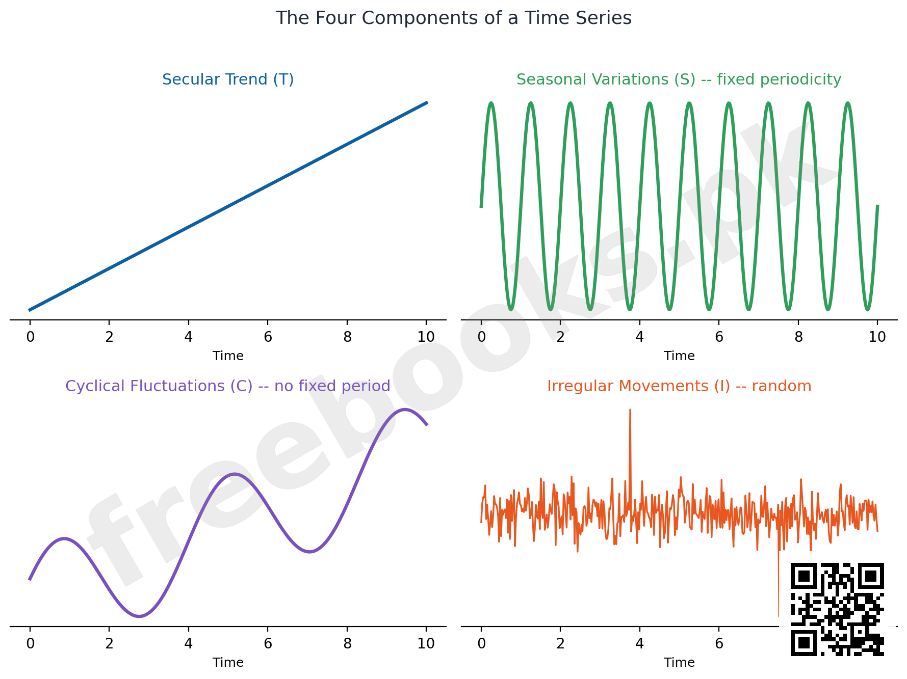
A time series may be composed of up to four distinct components, each the result of a well-defined but different underlying cause; a given series need not contain all four. The secular (long-term) trend, T, is a smooth, steady, gradual movement of the series in the same direction (up or down) over a fairly long period, reflecting forces such as population growth, technological change, or shifting long-run demand — for example the decline in death rate due to advances in science, or steadily rising demand for wheat as population grows.

Seasonal variations, S, are short-term movements that recur regularly, with a fixed periodicity of a year or less (daily, weekly, monthly, yearly) — caused by the calendar seasons, religious festivals, or social customs, such as increased electricity use in summer or an after-Eid sale spike. Cyclical fluctuations, C, are longer-term oscillations about the trend that recur over a period longer than a year but WITHOUT a fixed periodicity (unlike seasonal variations) — caused by the business cycle, which has four phases: trough (depression, the lowest point), expansion (recovery, the upswing), peak (boom/prosperity, the highest point), and recession (contraction, the downswing). Cyclical fluctuations are less predictable than seasonal variations or trend, making them more consequential for business planning.

Irregular movements, I, are unpredictable, unsystematic, non-recurring changes caused by random events such as wars, floods, earthquakes, strikes, or fires — also called erratic, accidental, or random variations.

16.3 Analysis of Time Series

Analysing a time series means decomposing it into its separate components for individual study, mainly to support estimation and forecasting. Two standard models combine the four components: the multiplicative model, Y=TxSxCxI, treats trend T in the series' original units while S, C, and I are unitless percentage index numbers; the additive model, Y=T+S+C+I, treats all four components in the series' original units. The multiplicative model is conventionally treated as the standard model for time series analysis.

Coded Time Variable: to simplify trend calculations, the time variable t is coded as x=(t-tbar)/h (or a rescaled version), where tbar=(first period + last period)/2 and h is the constant interval between periods. Since sum(t-tbar)=0 by construction, the coding guarantees sum(x)=0=sum(x^3)=sum(x^5)=…, which is what dramatically simplifies the least squares normal equations used later in the chapter. For an odd number of periods, x=0 is assigned to the exact middle period; for an even number of periods, x=0 falls halfway between the two middle periods (giving half-integer codes unless the unit of measurement is redefined as half a period, which restores whole-number codes).

16.4 Estimation of Secular Trend

Four methods are used to estimate secular trend, in increasing order of objectivity and mathematical rigour. The Method of Free Hand Curve plots the historigram and then draws, by eye, a smooth line or curve that best represents the general movement — often anchored through the point (mean time, mean y) for extra reliability. It is simple and quick, and smooths out seasonal variations, but is a rough, personally-biased method: different analysts will draw different lines from the same data.

The Method of Semi-Averages divides the observed series into two equal halves (omitting or duplicating the middle value if n is odd), computes the average of each half, and draws a straight line through the two resulting points, each plotted at its half's midpoint in time. Given the two semi-averages y1' (at x1) and y2' (at x2), the trend line's slope is b=(y2'-y1')/(x2-x1) and intercept a=y1'-b.x1; equivalently, for the whole series, b=4(S2-S1)/n^2 where S1, S2 are the sums of the first and second halves and n is the total number of periods. This method is objective and quick, and gives a better approximation than free hand curve (since it rests on a definite mathematical rule), but is heavily affected by extreme values (because it uses arithmetic means) and is only appropriate when the underlying trend is genuinely linear.

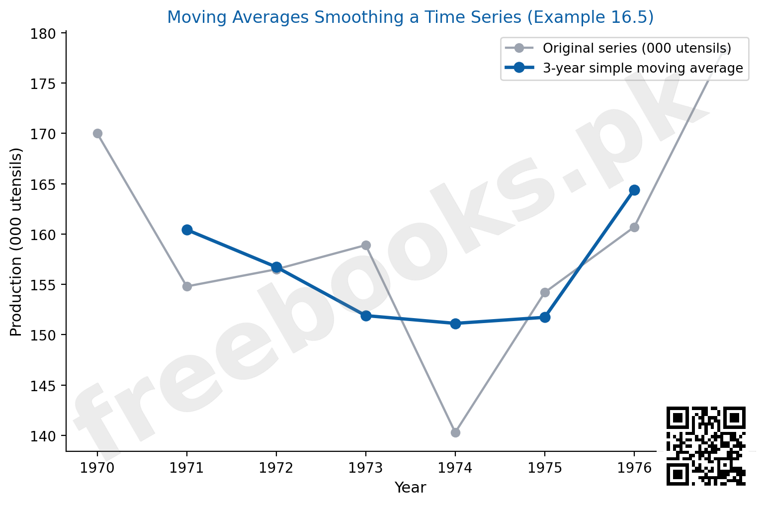
The Method of Moving Averages replaces each observation with the average of itself and a fixed number k of neighbouring periods, sliding this window one period at a time across the whole series: a1=(1/k)sum of the first k values, a2=(1/k)sum of values 2 through k+1, and so on; equivalently, using successive k-period totals S1, S2, S3,…, each new total is obtained from the previous one by dropping the oldest value and adding the next one, S2=S1+y_{k+1}-y1, and each average a_i=S_i/k. Each moving average is plotted against the MIDDLE of its k-period window. When k is odd, this middle falls exactly on an observed time period; when k is even, it falls between two periods, requiring a further 2-period 'centring' average of the moving averages themselves to realign them with the actual observed periods (yielding CENTRED moving averages). Moving averages smooth out periodic (seasonal/cyclical) fluctuations most effectively when the averaging period is chosen to match the periodicity of those fluctuations, but the method sacrifices trend values at both ends of the series, is still sensitive to extreme observations, and provides no actual mathematical equation for extrapolating the trend into the future.

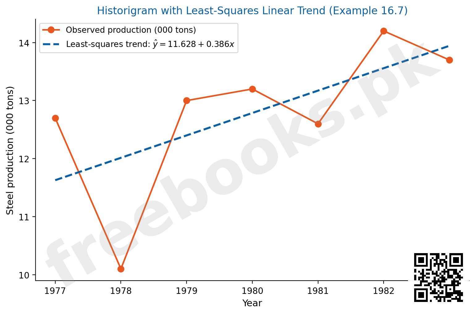
The Method of Least Squares fits a definite mathematical curve — typically a straight line y-hat=a+bx or a parabola y-hat=a+bx+cx^2, with x the coded time value — by minimizing the sum of squared deviations of observed values from the fitted curve, exactly the same least squares principle developed in Chapter 14 for ordinary regression. For a straight line, the normal equations sum(y)=na+b.sum(x) and sum(xy)=a.sum(x)+b.sum(x^2) give b=[n.sum(xy)-sum(x)sum(y)]/[n.sum(x^2)-(sum x)^2] and a=ybar-b.xbar; when the time variable has been coded so sum(x)=0, these collapse to the much simpler a=ybar=sum(y)/n and b=sum(xy)/sum(x^2). For a parabola, with x coded so sum(x)=0=sum(x^3), the normal equations similarly simplify to give c=[n.sum(x^2 y)-sum(x^2)sum(y)]/[n.sum(x^4)-(sum x^2)^2], a=[sum(y)-c.sum(x^2)]/n, and b=sum(xy)/sum(x^2). The fitted line/curve always passes through the point (xbar, ybar); the residuals sum to zero (sum y = sum y-hat); and the smaller the sum of squared residuals, the better the fit — which is exactly how a quadratic trend can be objectively confirmed to fit better than a linear one for a given dataset, by comparing their two sum(e^2) values directly.

Shifting the Origin: given an already-fitted trend line y-hat=a+bx (linear) with the origin at some reference time period, moving the origin k periods FORWARD means substituting (x+k) for x, and k periods BACKWARD means substituting (x-k) for x; only the intercept changes (to a+/-bk), never the slope b. For a quadratic trend, the same substitution is made into y-hat=a+bx+cx^2 and the result expanded and regrouped in powers of the new x, changing all three constants a, b, and c.

Important Definitions

Key Facts and Relations

Topic	Key Fact / Relation
Time series model	y = f(t) + e (f(t) = signal, e = noise)
Multiplicative and additive models	Multiplicative: Y = T x S x C x I; Additive: Y = T + S + C + I
Coded time variable (general)	x = (t – tbar)/h, tbar = (first period + last period)/2
Semi-averages trend slope and intercept	b = (y2' – y1')/(x2 – x1); a = y1' – b.x1; [b = 4(S2-S1)/n^2 for whole series]
k-period moving average (successive)	a1 = S1/k; a2 = a1 + (y_{k+1} – y1)/k; S2 = S1 + y_{k+1} – y1
Least squares linear trend (general)	b = [n.sum(xy) – sum(x)sum(y)] / [n.sum(x^2) – (sum x)^2]; a = ybar – b.xbar
Least squares linear trend (coded, sum x=0)	a = ybar = sum(y)/n; b = sum(xy)/sum(x^2)
Quadratic (parabolic) trend model	y-hat = a + bx + cx^2
Quadratic trend estimates (coded, sum x=0=sum x^3)	c = [n.sum(x^2 y) – sum(x^2)sum(y)] / [n.sum(x^4) – (sum x^2)^2]; a = [sum(y) – c.sum(x^2)]/n; b = sum(xy)/sum(x^2)
Shifting the origin (linear trend)	y-hat = a + b(x +/- k) = (a +/- bk) + bx
Sum of squared residuals (goodness of fit)	sum(e^2) = sum(y^2) – a.sum(y) – b.sum(xy) [linear]; minus c.sum(x^2 y) also, for quadratic
Properties of the least squares trend line	Passes through (xbar, ybar); sum(y – y-hat) = 0, so sum(y) = sum(y-hat)

Diagrams

The Four Components of a Time Series: A 4-panel illustration showing idealised patterns for each classical component: secular trend (a smooth rising straight line), seasonal variations (a regular repeating up-down wave pattern within each year), cyclical fluctuations (a longer, irregular-period wave oscillating around a rising trend), and irregular movements (a jagged, unpredictable random pattern with occasional spikes), illustrating how a real time series is the combination of some or all of these

Historigram with Least-Squares Linear Trend (Example 16.7): A historigram (line plot) of steel production 1977-1983, with the least-squares fitted straight trend line y-hat=11.628+0.386x overlaid, showing how the fitted line captures the general upward movement while smoothing over the year-to-year fluctuations

Moving Averages Smoothing a Time Series (Example 16.5): The original (jagged) yearly production series for silver utensils 1970-1977 plotted alongside its 3-year simple moving average, showing visually how the moving average smooths out short-term fluctuations to reveal the underlying movement, while losing values at both ends of the series

Short Questions & Answers

Long Questions & Answers

Describe the four classical components of a time series in detail, and explain how the multiplicative and additive models combine them, illustrating with realistic examples for each component.

What is the secular (long-term) trend component of a time series?

The secular or long-term trend, T, is the smooth, gradual, persistent movement of the series in one consistent direction over a fairly long span of time, reflecting slow-moving underlying forces that don't reverse from one period to the next. Examples include the long-run decline in death rates as medical science advances, steadily rising wheat demand as a population grows, and the gradual, sustained shift toward smaller, fuel-efficient cars over decades.

What are seasonal variations, and how do they differ from other components?

Seasonal variations, S, are short-term fluctuations that repeat with a fixed periodicity of one year or less, driven by causes tied to the calendar — physical seasons, festivals, or social customs. Examples include heavier weekend sales at a department store, a summer jump in electricity use from air conditioning, or a predictable post-Eid sales spike. The key diagnostic feature is that both the timing and roughly the size of the fluctuation repeat reliably and can be anticipated in advance.

What are cyclical fluctuations, and how do they differ from seasonal variations?

Cyclical fluctuations, C, are also recurring, wave-like oscillations around the trend, but unlike seasonal variation they lack a fixed periodicity — a business cycle might last two years in one instance and seven in another. Cycles move irregularly through four phases: a trough (lowest point), an expansion/recovery (upswing), a peak (highest point, or boom), and a recession/contraction (downswing). Because they lack a fixed rhythm, cyclical fluctuations are harder to forecast and riskier for planning than seasonal variations.

What are irregular movements, and how do the multiplicative and additive models combine all four components?

Irregular (erratic or accidental) movements, I, are whatever variation remains once trend, seasonal, and cyclical effects are accounted for — unpredictable, one-off disturbances like wars, floods, strikes, or fires, such as a steel strike delaying production for a week. The multiplicative model combines all four as Y = T x S x C x I, with T in original units and S, C, I expressed as unitless percentage indices; it is treated as the standard model. The additive model instead uses Y = T + S + C + I, with all four components expressed in original units.

Why is the multiplicative model generally preferred over the additive model?

The additive model assumes the absolute size of the seasonal, cyclical, and irregular fluctuations stays roughly constant regardless of the trend's level — often unrealistic for economic and business series, where fluctuations typically scale up proportionally as the trend level grows. Because the multiplicative model expresses S, C, and I as percentage indices that automatically scale with the trend, it better fits this common real-world pattern, which is why it has become the conventional default choice in practice.

Compare the four methods of estimating secular trend — free hand curve, semi-averages, moving averages, and least squares — explaining the mechanics, and the relative merits and demerits, of each, and explain why least squares is generally considered the most rigorous of the four.

How does the free hand curve method estimate trend, and what is its main weakness?

After plotting the historigram of the series, the analyst simply draws by eye a smooth line or curve through the data that seems to capture its general movement, ideally passing through the point representing the overall mean time and mean value. It is fast and requires no calculation, but is entirely subjective — two analysts working from the same data could draw two visibly different trend lines, with no principled way to say which one is more correct.

How does the method of semi-averages work, and what are its limitations?

The series is split into two equal halves, dropping or duplicating the middle value if the count is odd, the mean of each half is computed and plotted at that half's own midpoint in time, and a straight line is drawn connecting the two points using ordinary coordinate geometry. This is genuinely objective — any two analysts working from the same data arrive at exactly the same line — but it remains sensitive to extreme values within either half, and only works when the underlying trend is genuinely linear.

How does the method of moving averages work, and what are its drawbacks?

Each observation is replaced by the average of itself and a symmetric window of k neighbouring periods, with the window sliding forward one period at a time across the series. This averaging tends to cancel short-term seasonal and irregular noise while a genuine trend persists, provided k is matched to the actual periodicity being removed, such as a 12-month average to eliminate an annual pattern. Its drawbacks: no trend values can be computed near the start and end of the series, it stays sensitive to extreme observations, and it never produces an equation, so it cannot forecast future values.

How does the least squares method estimate trend, and why is it considered the most rigorous of the four methods?

Least squares fits a definite equation — usually a straight line y-hat=a+bx, or a quadratic y-hat=a+bx+cx^2 when a straight line fails to capture visible curvature — chosen so the sum of squared deviations between observed and fitted values is as small as possible, the same principle used for two-variable regression, with coded time as the independent variable. Because it produces a definite equation rather than a hand-drawn line or a table of local averages, it can compute a precise trend value at any period AND extrapolate forward to genuine forecasts, and different candidate models can be objectively compared by their sums of squared residuals — a rigour the other three methods cannot match.

Multiple Choice Questions (MCQs)

Quick Revision Summary

• Time series: y=f(t)+e, signal f(t) + noise e; historigram = time-series line graph
• 4 components: Secular trend (T, long-term smooth) | Seasonal (S, fixed periodicity <=1yr) | Cyclical (C, no fixed periodicity, business cycle) | Irregular (I, random/unpredictable)
• Business cycle phases: trough -> expansion -> peak -> recession
• Multiplicative: Y=TxSxCxI (T in original units, S/C/I unitless %) | Additive: Y=T+S+C+I (all original units)
• Coded time variable: x=(t-tbar)/h chosen so sum(x)=0=sum(x^3), simplifying least squares
• Free hand curve: quick but subjective/biased | Semi-averages: objective but only for linear trend, sensitive to extremes
• Moving averages: smooth out fixed-period fluctuations; no trend values at ends; no forecasting equation
• Least squares linear: b=sum(xy)/sum(x^2), a=ybar (when sum x=0) | Quadratic: adds c=[n.sum(x^2y)-sum(x^2)sum(y)]/[n.sum(x^4)-(sum x^2)^2]
• Best-fit model = smaller sum(e^2) = sum(y^2)-a.sum(y)-b.sum(xy)[-c.sum(x^2y)]
• Shifting origin (linear): only intercept changes, a+/-bk; slope b unchanged

Exam Tips

• Always draw the historigram first — visual inspection tells you whether to expect a linear or curved trend before you compute anything
• Remember: seasonal = FIXED periodicity, cyclical = NO fixed periodicity — this is the single most-tested distinction in this chapter
• When n is even and using semi-averages, the two midpoint x-values (x1, x2) will be at the centre of each half, not at integer years — don't forget this when computing b=(y2'-y1')/(x2-x1)
• For moving averages, always double-check whether k is odd (no centring needed) or even (must centre with a further 2-period average)
• When coding time for least squares, decide up front whether the unit is 1 year or 1/2 year for EVEN numbers of periods — this changes b (but not the trend values themselves) by a factor of 2
• To compare linear vs quadratic fits, compute BOTH sum(e^2) values and pick the smaller one — don't just eyeball which curve 'looks' better