Statistics 2nd Year Chapter 11: Sampling Techniques and Sampling Distributions Notes (PDF Download)

Almost nothing in real-world statistics is based on studying an entire population — it is far too slow, expensive, or simply impossible. Instead, statisticians study a carefully chosen sample and use it to draw conclusions about the whole population. This chapter builds the foundation for that entire process: how populations and samples are defined, how a representative sample is actually selected (probability vs non-probability methods, simple random sampling, stratified sampling), and what kinds of errors can creep in along the way.

The second and more theoretical half of the chapter introduces sampling distributions — the probability distribution of a statistic (like the sample mean or sample proportion) across all possible samples of a given size. This concept, and especially the Central Limit Theorem introduced here, is the single most important theoretical bridge in the entire course: it is what allows the normal distribution from Chapter 10 to be used for inference about sample means and proportions in every chapter that follows (Estimation, Hypothesis Testing).

Learning Objectives

• Define population, sample, sampling, parameter, and statistic, and distinguish clearly between each pair
• Distinguish probability sampling from non-probability sampling and describe common methods of each
• Explain and apply simple random sampling with and without replacement, including counting the number of possible samples
• Describe stratified sampling and explain when it is preferred over simple random sampling
• Distinguish sampling error from non-sampling error, and define accuracy, precision, and bias
• Explain what a sampling distribution of a statistic is and define its standard error
• State and apply the properties of the sampling distribution of the sample mean, with and without the finite population correction
• State the Central Limit Theorem and explain its importance in statistical inference
• Find the mean and standard error of the sampling distributions of the difference of two means, sample proportion, difference of two proportions, and sample variance

Key Concepts

11.1-11.2 Population and Sample

A population is the totality of all observations (or all sampling units) possessing some common, specified characteristic that a researcher wants to study — it may be finite (a limited, countable number of units, such as all registered voters in a city) or infinite (an unlimited number of units, such as all possible outcomes of tossing a coin indefinitely, or all items that could ever be produced by an ongoing production process).

A sample is a part of the population selected in such a way that it is expected to represent the characteristics of the whole population reasonably well. Sampling is the procedure used to select such a representative sample. A sample survey studies only a part of the population, whereas a census (complete enumeration) studies every single unit. Samples are generally preferred over a census because they save time, cost far less, are often more feasible for large or inaccessible populations, and — perhaps counter-intuitively — can sometimes give MORE accurate results than a census, since a smaller, well-managed data collection effort allows more careful measurement and closer supervision, reducing non-sampling errors. The limitations of sampling are that it can never give perfectly exact results (only estimates) and requires careful, expert planning to avoid a biased or unrepresentative sample.

11.3 Sampling Design

A sampling design is the complete plan for selecting a sample from a given population. Its building blocks are the sampling unit (the individual element, or group of elements, that will actually be selected, e.g., a household, a student, a factory) and the sampling frame — a complete list of all sampling units in the population, from which the sample is actually drawn (e.g., a voter list, a list of registered students). A good sampling frame should be accurate, complete, and up to date; a poor frame is one of the most common sources of non-sampling error.

Sampling methods fall into two broad families: non-probability sampling, in which the chance of any particular element being included in the sample cannot be determined in advance (examples include convenience sampling, judgment/purposive sampling, and quota sampling) — these are quick and cheap but their results cannot be generalized to the population with a known level of confidence; and probability sampling (also called random sampling), in which every element of the population has a known, non-zero probability of being selected. Probability sampling is the standard for scientific inference because it allows the sampling error to be objectively measured and controlled. Selection may be done with replacement (a selected unit is returned to the population and can be chosen again) or without replacement (a selected unit is removed and cannot be chosen again).

11.6 Simple Random Sampling

Simple random sampling (SRS) is the most basic probability sampling method: a sample of size n is drawn from a population of size N such that every possible sample of that size has an equal chance of being selected. It can be carried out physically using the lottery method (writing all N units on identical slips, mixing thoroughly, and drawing n of them) or, more commonly and more rigorously, using a table of random numbers (or a random-number generator), where units of the population are numbered and n numbers are read off the table according to a fixed, unbiased rule.

Theorem 11.1 gives the counting rule that underlies every sampling-distribution calculation in this chapter: if sampling is done WITH replacement, the number of possible ordered samples of size n from a population of size N is N raised to the power n (N^n) — because each of the n draws independently has N possible outcomes. If sampling is done WITHOUT replacement, the number of possible ordered samples of size n is N(N-1)(N-2)…(N-n+1), written compactly as NPn (N permute n) — because the first draw has N possible outcomes, the second has only N-1 remaining, the third only N-2, and so on, since a selected unit cannot be chosen again. These two counting formulas (N^n and NPn) are the starting point of virtually every worked example on sampling distributions in this chapter — they tell you exactly how many rows the sampling distribution table will have before you even start building it.

11.7 Stratified Sampling

Stratified sampling is used when the population is heterogeneous but can be divided into non-overlapping, internally homogeneous subgroups called strata (for example, dividing a student population into strata by grade level, or a national population into strata by province). A simple random sample is then drawn independently from each stratum, and the stratum samples are combined into the final overall sample. Stratified sampling is preferred over plain SRS whenever the strata differ meaningfully from each other but units within the same stratum are fairly similar, because it guarantees representation from every subgroup and typically produces estimates with a smaller standard error than an SRS of the same total size drawn from the unstratified population.

11.8 Errors in Sampling

No sample-based estimate is ever perfectly exact; the discrepancy between an estimate and the true population value can arise from two very different sources. Sampling error is the difference E = T – theta between a sample statistic T (such as the sample mean) and the true population parameter theta (such as the population mean) that arises purely because only a sample, and not the entire population, was observed — it exists even if every single measurement in the sample was made perfectly, and it can generally be reduced by increasing the sample size. Non-sampling errors, by contrast, can occur even in a complete census, and arise from sources such as faulty questionnaire design, non-response, data-entry mistakes, or interviewer bias — these do NOT necessarily shrink as the sample size grows, and in fact tend to grow more troublesome in very large surveys where quality control becomes harder to maintain.

Two further concepts describe the quality of an estimate. Accuracy refers to how close an estimate is to the true population value — a highly accurate estimate has very little sampling error. Precision refers to how closely repeated estimates (from repeated samples of the same size and design) cluster around each other, regardless of whether they are close to the true value — it is measured by the standard error of the estimator; a small standard error means high precision. Bias is defined as the difference between the expected value of an estimator T and the true parameter, Bias = E(T) – theta; an unbiased estimator has Bias = 0, meaning it is correct 'on average' across all possible samples, even though any single sample estimate may still differ from the true value due to ordinary sampling error.

11.9-11.10 Parameters, Statistics, and the Idea of a Sampling Distribution

A parameter is any descriptive numerical measure calculated from the ENTIRE population — since the population is fixed, a parameter is a constant with one single true (though often unknown) value. Key parameters include the population total tau = sum of all x-j, the population mean mu = tau/N, the population variance sigma-squared = [sum of (x-j – mu)^2]/N, and the population proportion pi = k/N (where k is the number of elements possessing some attribute).

A statistic is any descriptive numerical measure calculated from a SAMPLE — because the particular sample drawn will differ from one instance to the next, a statistic is a random variable, taking a different value for each possible sample; it therefore has its own probability distribution. Key statistics include the sample total (sum of x-i), the sample mean x-bar = (sum of x-i)/n, the sample proportion p = x/n, and two versions of sample variance: the divide-by-n version s-squared = [sum of (x-i – x-bar)^2]/n and the divide-by-(n-1) version s-hat-squared = [sum of (x-i – x-bar)^2]/(n-1) — the two are related by n.s^2 = (n-1).s-hat^2.

The sampling distribution of a statistic is the probability distribution formed by the values of that statistic computed from EVERY possible sample of a given size that could be drawn from the population. The standard error of a statistic is defined as the standard deviation of its sampling distribution — it measures how much the statistic is expected to vary from one random sample to the next, and it is the single most important number needed for statistical inference (confidence intervals and hypothesis tests, covered in the next two chapters) because it quantifies the precision of an estimate.

11.11-11.12 Sampling Distribution of the Sample Mean and the Central Limit Theorem

The sampling distribution of the sample mean X-bar is the probability distribution of the means of all possible simple random samples of size n drawn from a population with mean mu and variance sigma-squared. Its properties are given by a sequence of theorems. Theorem 11.2: the mean of the sampling distribution of X-bar always equals the population mean, mu-Xbar = E(X-bar) = mu, regardless of sample size or replacement method — so X-bar is an unbiased estimator of mu. Theorem 11.3: when sampling is done with replacement from an infinite population (or a finite one with replacement), the variance of X-bar is the population variance divided by the sample size, sigma-Xbar-squared = sigma-squared/n, so the standard error is sigma-Xbar = sigma/sqrt(n) — notice the standard error shrinks as the sample size n grows, which is exactly why larger samples give more precise estimates.

Theorem 11.4 extends this to sampling WITHOUT replacement from a finite population of size N: the variance picks up an extra multiplier called the finite population correction (fpc), sigma-Xbar-squared = (sigma-squared/n).[(N-n)/(N-1)]. The fpc is always less than or equal to 1, so sampling without replacement always gives an equal or SMALLER standard error than sampling with replacement — and when the sample size n is small relative to the population size N (a small 'sampling fraction' n/N), the fpc is so close to 1 that it can often be safely ignored in practice.

Theorem 11.5 states that if the ORIGINAL population itself is normally distributed, then X-bar is exactly normally distributed with mean mu and variance sigma-squared/n, for ANY sample size (even n=1). But most real populations are not normal — which is where Theorem 11.6, the Central Limit Theorem (CLT), becomes indispensable: for a LARGE sample size, the sampling distribution of X-bar is approximately normal with mean mu and variance sigma-squared/n, REGARDLESS of the shape of the original population's distribution. The larger the sample size, the better this normal approximation becomes. This is the single most powerful and far-reaching result in this chapter: it means the standardized variable Z = (X-bar – mu)/(sigma/sqrt(n)) can be treated as approximately standard normal even when nothing at all is known about the shape of the underlying population — and it is this fact alone that makes the confidence intervals and hypothesis tests of Chapters 12 and 13 possible for virtually any kind of data.

11.13 Sampling Distribution of the Difference Between Two Sample Means

When comparing two populations (for example, comparing the average lifetime of light bulbs from two different manufacturers), we work with the difference X-bar-1 minus X-bar-2 between two INDEPENDENT sample means. Theorem 11.7: the mean of this difference always equals the difference of the population means, mu = mu-1 – mu-2. Theorem 11.8: for independent samples with replacement (or from infinite populations), the variance of the difference is the SUM of the two individual sampling variances, sigma-squared = sigma-1-squared/n-1 + sigma-2-squared/n-2 — variances of independent random variables add even though we are taking a DIFFERENCE, because Var(A-B) = Var(A) + Var(B) when A and B are independent. Theorem 11.9 adds the finite population correction to each term for sampling without replacement from finite populations, and Theorem 11.10 confirms that if both original populations are normal, the difference X-bar-1 – X-bar-2 is exactly normally distributed (and by the Central Limit Theorem, approximately normal for large samples even if the populations are not normal).

11.14-11.15 Sampling Distribution of Sample Proportion and Its Difference

When the characteristic of interest is qualitative with two outcomes (success/failure, yes/no), the population proportion is pi = k/N and the sample proportion is P = X/n, where X counts the number of 'successes' in the sample. Theorem 11.11: for sampling with replacement (or from an infinite/Bernoulli population), P has mean mu-P = pi and variance sigma-P-squared = pi(1-pi)/n — in fact the exact sampling distribution of P in this case is directly linked to the binomial distribution from Chapter 9. The shape of the sampling distribution of P is right-skewed when pi < 0.5, left-skewed when pi > 0.5, and symmetric when pi = 0.5, but as n grows large it approaches a normal shape by the Central Limit Theorem. Theorem 11.12 adds the finite population correction for sampling without replacement, linking the sampling distribution of P in that case to the hypergeometric distribution, also from Chapter 9.

Just as with means, we often compare two proportions from two independent Bernoulli populations. Theorem 11.13: the mean of the difference P1 – P2 equals pi-1 – pi-2. Theorem 11.14: for independent samples with replacement, the variance of the difference is again the sum of the two individual variances, sigma-squared = pi-1(1-pi-1)/n-1 + pi-2(1-pi-2)/n-2. Theorem 11.15 adds the finite population correction to each term for sampling without replacement from finite populations.

11.16-11.17 Other Sampling Distributions: Sample Variance

Besides the mean and the proportion, every other sample statistic — the sample median, the sample variance, the sample standard deviation — has its own distinct sampling distribution, and a full specification of any sampling distribution must always state three things together: the population being sampled, the particular statistic being computed, and the sample size being used, since changing any one of these three produces a genuinely different sampling distribution. For the sample variance S-squared = [sum of (X-i – X-bar)^2]/n (computed with the divide-by-n convention), the sampling distribution has the property mu-S-squared = E(S-squared) = [(n-1)/n].sigma-squared — notice this is slightly LESS than the true population variance sigma-squared, which is exactly why the alternative divide-by-(n-1) version of sample variance is preferred as an unbiased estimator in later chapters on estimation.

Important Definitions

Key Facts and Relations

Topic	Key Fact / Relation
Population parameters	mu = (sum x_j)/N; sigma^2 = (sum x_j^2)/N – mu^2; pi = k/N
Sample statistics	x-bar = (sum x_i)/n; s^2 = [sum(x_i – x-bar)^2]/n; p = x/n
Number of samples (Theorem 11.1)	With replacement: N^n | Without replacement: NPn = N(N-1)…(N-n+1)
Mean of X-bar (Thm 11.2)	mu_Xbar = E(X-bar) = mu
Variance of X-bar, with replacement (Thm 11.3)	sigma_Xbar^2 = sigma^2/n; SE = sigma/sqrt(n)
Variance of X-bar, without replacement (Thm 11.4)	sigma_Xbar^2 = (sigma^2/n).[(N-n)/(N-1)]
Central Limit Theorem (Thm 11.6)	For large n: X-bar ~approx N(mu, sigma^2/n), regardless of population shape
Z for sample mean	Z = (X-bar – mu)/(sigma/sqrt(n))
Difference of means: mean & variance (Thm 11.7-11.8)	mu = mu1-mu2; sigma^2 = sigma1^2/n1 + sigma2^2/n2
Sample proportion: mean & variance (Thm 11.11-11.12)	mu_P = pi; sigma_P^2 = pi(1-pi)/n [x fpc if without replacement]
Difference of proportions: mean & variance (Thm 11.13-11.14)	mu = pi1-pi2; sigma^2 = pi1(1-pi1)/n1 + pi2(1-pi2)/n2
Mean of sample variance (S^2, divide by n)	mu_(S^2) = E(S^2) = [(n-1)/n].sigma^2

Diagrams

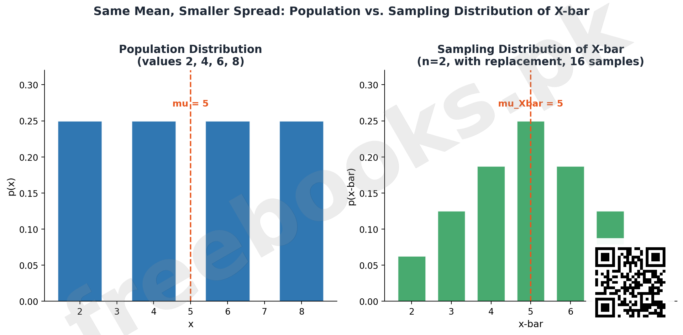
Population Distribution vs. Sampling Distribution of the Mean: A side-by-side comparison of a flat (uniform) population distribution for the values 2,4,6,8 against the mound-shaped sampling distribution of the sample mean for all 16 possible samples of size 2 drawn with replacement — both centred at the same mean of 5, but the sampling distribution of X-bar is visibly narrower, illustrating Theorem 11.2 (equal means) and Theorem 11.3 (reduced variance)

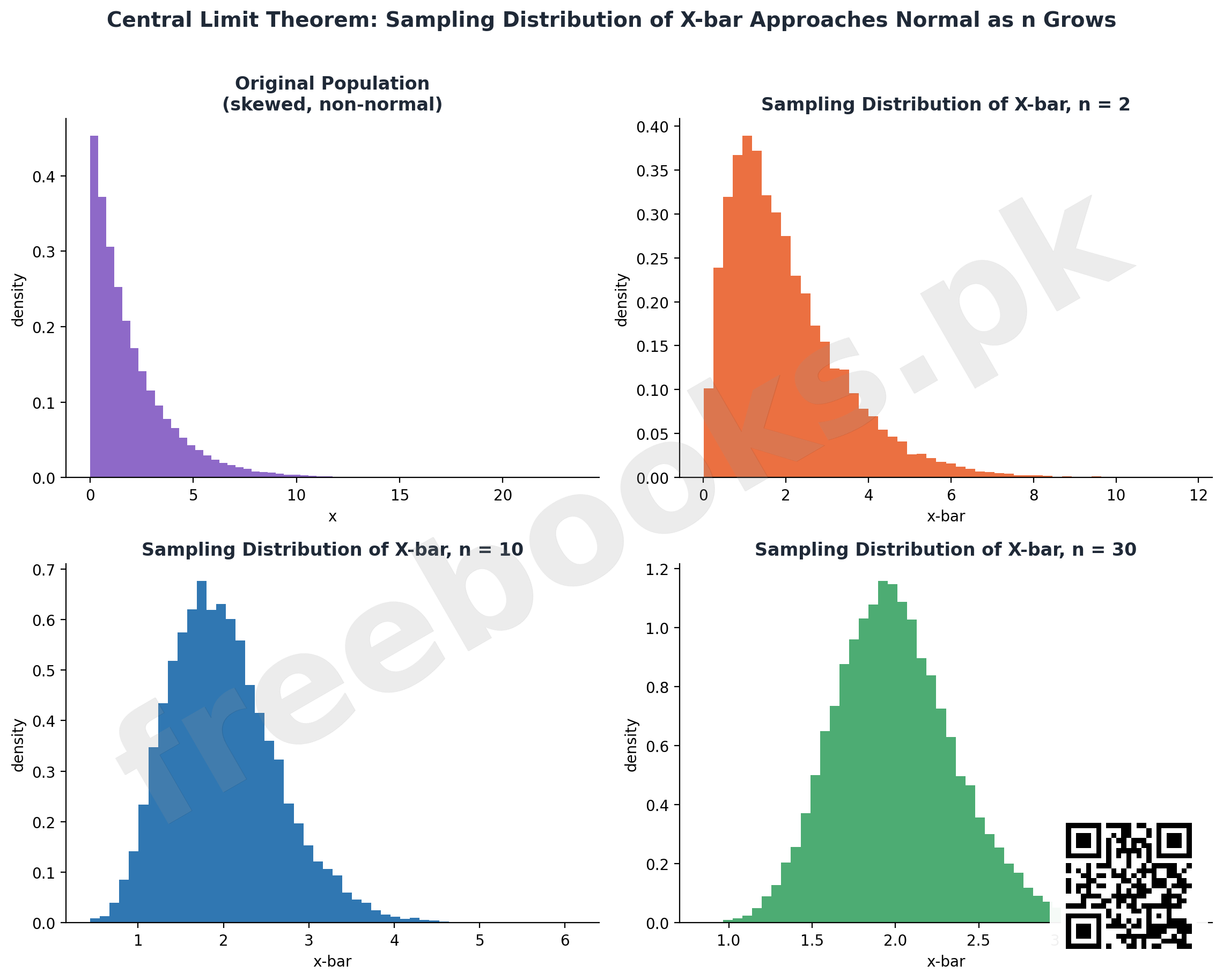
The Central Limit Theorem in Action: Three panels showing a skewed (non-normal) population distribution alongside simulated sampling distributions of the sample mean for increasing sample sizes n=2, n=10, and n=30, illustrating how the sampling distribution of X-bar becomes progressively more bell-shaped and narrower as n grows, regardless of the population's original skewed shape

Effect of the Finite Population Correction Factor: A line chart showing the standard error of the sample mean against sample size n for a fixed population size N, comparing the with-replacement formula sigma/sqrt(n) against the without-replacement formula that includes the finite population correction, showing how the fpc pulls the standard error down further as the sample size approaches the population size

Short Questions & Answers

Long Questions & Answers

Explain the concept of a sampling design, distinguishing probability from non-probability sampling, and describe simple random sampling and stratified sampling as two concrete probability sampling methods.

What is a sampling design, and what are its two key building blocks?

A sampling design is the deliberate plan governing how a sample will be selected from a population. It rests on two foundations: the sampling unit, the individual element actually selected, and the sampling frame, the complete list of every unit that exists within the population under study. If the sampling frame is inaccurate or incomplete, it becomes the single most common source of non-sampling error in a survey, regardless of how carefully the actual selection procedure is carried out afterward.

How does probability sampling differ from non-probability sampling?

In non-probability sampling, the probability of any particular individual being included in the sample cannot be calculated in advance; common examples include convenience sampling and quota sampling, where a researcher's own judgment decides which units to include. Because the underlying probability of selection is unknown, results cannot be legitimately generalized back to the wider population. Probability sampling, by contrast, gives every unit a known, non-zero probability of selection, which is what allows sampling error to be objectively measured and controlled — making it the accepted foundation for serious statistical inference.

What is simple random sampling (SRS)?

Simple random sampling is the most basic probability method: a sample of size n is drawn from a population of size N so that every possible sample of that size has an equal chance of being selected. In practice this is done by the lottery method (drawing n slips from a mixed set of N) or, more commonly, using a random-number table or generator, with each unit assigned a unique number. When sampling is with replacement, the number of possible ordered samples is N^n; when sampling is without replacement, it is N(N-1)(N-2)…(N-n+1), denoted NPn.

What is stratified sampling, and when is it preferred over SRS?

Stratified sampling divides a heterogeneous population into distinct, non-overlapping strata that are internally more homogeneous — such as by province or grade level — and then draws an independent simple random sample from each stratum, combining them into the final sample. It is preferable to an unstratified SRS of the same overall size whenever the strata differ substantially from each other, because it guarantees every relevant subgroup is represented and typically produces estimates with a smaller standard error than an equivalently-sized unstratified sample.

State the Central Limit Theorem in full, and explain its relationship to Theorems 11.2 through 11.5 on the sampling distribution of the sample mean, including why it is considered the single most important theoretical result of this chapter.

What does Theorem 11.2 say about the mean of the sampling distribution of X-bar?

Theorem 11.2 states that regardless of the sample size n, and regardless of whether sampling is with or without replacement, the mean of the sampling distribution of the sample mean X-bar always equals the true population mean: mu-Xbar = E(X-bar) = mu. This has an important practical implication: X-bar is an unbiased estimator of mu. Any single sample's mean will typically differ somewhat from mu due to sampling error, but averaged across every conceivable sample, X-bar lands exactly on mu with no systematic bias.

What do Theorems 11.3 and 11.4 say about the variance of X-bar under sampling with and without replacement?

For sampling with replacement, Theorem 11.3 gives Var(X-bar) = sigma^2/n, so the standard error is sigma-Xbar = sigma/sqrt(n); as n increases this standard error shrinks, which is why larger samples give more precise estimates. For sampling without replacement from a finite population, Theorem 11.4 introduces the finite population correction factor (N-n)/(N-1), which is always <= 1 whenever n < N, and this factor further shrinks the standard error compared to sampling with replacement of the same size.

What does Theorem 11.5 say about exact normality of X-bar, and what is its key limitation?

Theorem 11.5 states that if the original population is itself normally distributed, then X-bar is exactly normally distributed with mean mu and variance sigma^2/n, and this holds for any sample size, even n=1. Its key limitation is that this exact result depends entirely on the population already being normal — an assumption that, in most real-world situations, either cannot be verified with confidence or can be shown to be false.

What does the Central Limit Theorem (Theorem 11.6) state, and how does it remove Theorem 11.5's limitation?

The Central Limit Theorem states that for a sufficiently large sample size, the sampling distribution of X-bar is approximately normal with mean mu and variance sigma^2/n, regardless of the shape of the original population — skewed, uniform, bimodal, or otherwise. The approximation improves as the sample size grows, generally becoming good around n=30 or more. This removes Theorem 11.5's restrictive requirement that the population itself be normal.

Why is the Central Limit Theorem considered the most important result of this chapter?

Because it removes the normal-population assumption, the Central Limit Theorem allows the standardized variable Z = (X-bar – mu)/(sigma/sqrt(n)) to be treated as approximately standard normal for large samples drawn from virtually any population. This single fact is what makes it possible to construct valid confidence intervals and conduct valid hypothesis tests for an unknown population mean using standard-normal-based methods — directly connecting the probability theory of earlier chapters to the estimation and hypothesis-testing methods that follow.

Multiple Choice Questions (MCQs)

Quick Revision Summary

• Population = whole group (parameter, constant); Sample = part studied (statistic, random variable)
• Sampling frame = list of all sampling units; probability sampling gives every unit a known chance of selection
• Theorem 11.1: with replacement N^n samples; without replacement NPn = N(N-1)…(N-n+1) samples
• Sampling error: T-theta, shrinks with larger n | Non-sampling error: from bad frames/questions/entry, doesn't shrink with n
• Accuracy = closeness to true value | Precision = closeness of repeated estimates (measured by SE) | Bias = E(T)-theta
• Thm 11.2-11.3: mu_Xbar=mu; sigma_Xbar^2=sigma^2/n (with replacement)
• Thm 11.4: without replacement, multiply variance by fpc = (N-n)/(N-1), always <=1
• Thm 11.6 (CLT): for large n, X-bar ~approx N(mu, sigma^2/n) regardless of population shape
• Difference of means: mu=mu1-mu2, sigma^2=sigma1^2/n1+sigma2^2/n2 (variances ADD for independent samples)
• Sample proportion: mu_P=pi, sigma_P^2=pi(1-pi)/n [x fpc if without replacement]

Exam Tips

• Always identify FIRST whether sampling is with or without replacement — it changes both the counting formula (N^n vs NPn) and the variance formula (fpc or not)
• When a question says 'infinite population' or doesn't mention N, treat it as sampling with replacement — no fpc needed
• For difference-of-means or difference-of-proportions problems, remember variances ADD even though you're computing a difference
• Build the sampling distribution table systematically: list all samples, compute the statistic for each, then tally into a frequency/probability table before computing mean and variance
• The CLT applies to means and proportions for LARGE n — don't assume normality for small samples unless the population itself is stated to be normal
• Double-check verification questions (e.g., 'verify mu_Xbar = mu') by computing both sides independently and confirming they match numerically