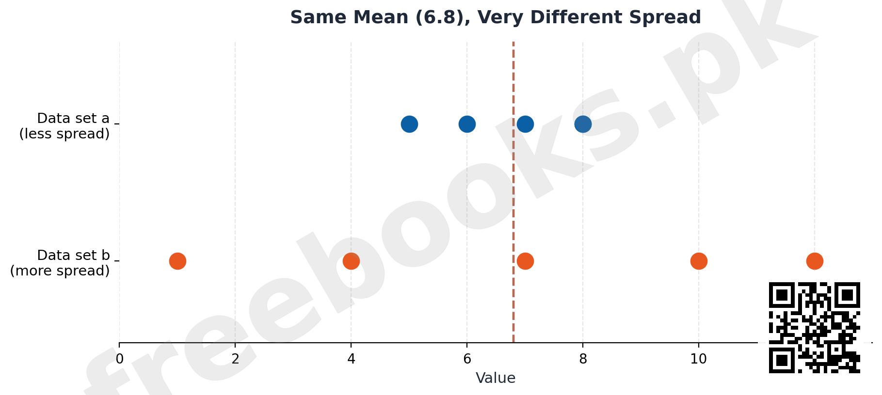
A measure of central tendency alone does not tell us anything about how spread out the values in a data set are. Two data sets can share the exact same mean while differing enormously in their variability — for example, the sets 8, 7, 5, 8, 6 and 1, 4, 7, 10, 12 both have a mean of 6.8, yet the second set is clearly far more spread out than the first. To give a fuller description of data, we need a numerical quantity called a measure of dispersion (or variability) that captures this spread.
This chapter covers the common absolute measures of dispersion — range, quartile deviation, mean deviation, variance, and standard deviation — which carry the same units as the original data, along with relative measures such as the coefficient of variation, which are unit-free ratios useful for comparing the variability of different data sets. It also introduces moments as a more general tool for describing a distribution's shape, and uses them to define skewness (lack of symmetry) and kurtosis (peakedness and tail length).
Learning Objectives
- Explain why a measure of central tendency alone is insufficient to describe a data set
- Calculate range and quartile deviation for ungrouped and grouped data
- Calculate mean deviation from the mean and from the median
- Calculate variance and standard deviation using the direct and short-cut (coding) formulas
- State and apply the key properties of variance and standard deviation, including for combined data sets
- Calculate the coefficient of variation and other relative measures of dispersion
- Define moments about the mean, about an arbitrary origin, and about zero, and relate them to variance
- Explain skewness and calculate Karl Pearson's and Bowley's coefficients of skewness
- Explain kurtosis and distinguish mesokurtic, platykurtic, and leptokurtic distributions
Key Concepts
4.1 Introduction
Two data sets with vastly different variability can still share the same measure of central tendency, which shows that central tendency alone is not sufficient to describe a data set. A measure of dispersion (or variability) is a numerical quantity that describes how spread out the values in a data set are. There are two broad types: absolute measures, which carry the same units as the original data (range, quartile deviation, mean deviation, variance, and standard deviation), and relative measures, which are unitless ratios (discussed under coefficient of variation).
4.1.1 Range
The range of n values is the difference between the largest and smallest observation: R = Y(n) – Y(1). For grouped data, the range is calculated as the mid-value of the highest class minus the mid-value of the lowest class. Merits: very easy to calculate, and useful for small samples. Demerits: not based on all the observations, and depends only on the two most extreme values, making it highly sensitive to outliers.
4.1.2 Quartile Deviation
Quartile deviation (Q.D), also called the semi-interquartile range, is based on the first and third quartiles: Q.D = (Q3 – Q1) / 2. It can never be negative, since Q3 is always at least as large as Q1; a small Q.D indicates low variability, and a large Q.D indicates high variability. The coefficient of quartile deviation, a relative (unit-free) measure, is calculated as (Q3 – Q1) / (Q3 + Q1). Merits: easy to calculate, and not affected by extreme observations. Demerits: not based on all the observations, and two different distributions can share identical quartiles and therefore identical Q.D despite otherwise differing.
4.1.3 Mean Deviation
Mean deviation (M.D) is the mean of the absolute deviations of observations from the mean, median, or mode: M.D = (sum of |Y – M|) / n, where absolute deviations means all deviations are treated as positive. For grouped data, M.D = (sum of fi|Yi – M|) / (sum of fi). Key properties: mean deviation from the median is always the smallest possible mean deviation (smaller than from any other value); M.D is always greater than or equal to zero; and for symmetrical distributions, M.D = (4/5) times the standard deviation. Merits: easy to calculate, and based on all the observations. Demerits: affected by extreme values, not readily suited to further mathematical development, and it discards the sign of each deviation, losing information about direction.
4.1.4 Variance and Standard Deviation
Variance is the mean of the squared deviations of all observations from their mean. The population variance is denoted sigma-squared; the sample variance, denoted S-squared, is calculated as the sum of squared deviations from the sample mean divided by n (or, for grouped data, weighted by frequency). A short-cut formula avoids computing deviations directly: S-squared equals the mean of the squared values minus the square of the mean. Variance is based on all the observations, easy to calculate and understand, but is affected by extreme values.
Standard deviation (S) is the positive square root of variance, restoring the original units of measurement that variance's squaring operation removes. It has several important properties: the variance and standard deviation of a constant are zero; they are unaffected by adding or subtracting a constant from every observation (independent of origin); multiplying every observation by a constant a multiplies the variance by a-squared and the standard deviation by |a|; for two independent variables, the variance of their sum or difference equals the sum of their individual variances; and the combined variance of several groups can be calculated from each group's own variance, mean, and size, and the overall combined mean.
4.2 Coefficient of Variation and Other Relative Measures
The coefficient of variation (C.V) is the most widely used relative measure of dispersion: C.V = (S / mean) x 100 for a sample, or (sigma / mu) x 100 for a population. Because it is a ratio of two quantities with the same units, C.V is dimensionless and unaffected by the unit of measurement used — the same data will give the same C.V whether measured in millimeters, centimeters, or meters. A lower C.V indicates a comparatively more consistent (less variable relative to its mean) group, which makes C.V especially useful for comparing the variability of two or more data sets that may have very different means or units. Other relative measures include the coefficient of range, coefficient of quartile deviation, mean coefficient of dispersion (M.D divided by mean), median coefficient of dispersion (M.D divided by median), and coefficient of standard deviation (S divided by mean).
4.3 Moments
Measures of location and dispersion describe a data set's centre and spread, but tell us nothing about its shape. Moments are a family of measures used to describe shape. The rth moment about the mean (a central moment), denoted mr, is the mean of the rth powers of deviations from the mean. The first moment m1 is always zero; the second moment m2 is identical to the variance; the third moment m3 relates to skewness; and the fourth moment m4 relates to kurtosis (peakedness). Moments about an arbitrary origin a (raw or non-central moments), denoted mr-prime, are often easier to calculate directly and can be converted into moments about the mean using standard conversion relations — this is especially useful for grouped data with equal class widths, where a coding variable u = (y – a)/h simplifies the arithmetic considerably. When calculating moments from grouped data, choosing class midpoints introduces a small grouping error in the second and fourth moments in particular; Sheppard's corrections adjust for this when the frequency curve tapers gradually at both ends.
4.5 Skewness
Skewness refers to a lack of symmetry in a distribution. A distribution is symmetrical when mean, median and mode coincide and the frequency curve mirrors itself around the mean; otherwise it is skewed. A positively skewed distribution has a longer tail extending to the right; a negatively skewed distribution has a longer tail extending to the left. Extreme skewness produces J-shaped distributions. Several numerical measures quantify skewness: Karl Pearson's first coefficient, (Mean – Mode) / S; Karl Pearson's second coefficient, 3(Mean – Median) / S; and Bowley's coefficient, based on quartiles, (Q1 + Q3 – 2 x Median) / (Q3 – Q1), which lies between -1 and +1. All of these coefficients are zero for a perfectly symmetrical distribution, negative for negative skew, and positive for positive skew. The moment-based measure root-beta-1 (= m3 / (m2 raised to the power 1.5)) serves the same purpose: zero indicates symmetry, negative indicates negative skew, positive indicates positive skew.
4.5.1 Kurtosis
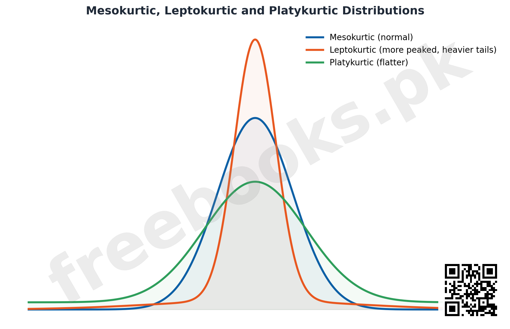
Kurtosis describes the peakedness of a distribution and the length of its tails. A mesokurtic distribution is the standard, normally-peaked shape. A leptokurtic distribution is more sharply peaked, with more values clustered close to the mean and also more values out in the tails. A platykurtic distribution is comparatively flatter, with more values spread between the mean and the tails than a mesokurtic distribution would have. Kurtosis is commonly assessed using the fourth moment about the mean relative to the square of the second moment (the variance).
Important Definitions
What is a measure of dispersion?
A numerical quantity that describes how spread out or variable the values in a data set are, complementing a measure of central tendency.
What is the difference between absolute and relative measures of dispersion?
Absolute measures carry the same units as the original data (e.g., range, standard deviation); relative measures are unit-free ratios (e.g., coefficient of variation), useful for comparing variability across different units or scales.
What is the range?
The difference between the largest and smallest observation in a data set: R = Y(n) – Y(1).
What is quartile deviation?
Half the difference between the third and first quartiles: Q.D = (Q3 – Q1) / 2, also called the semi-interquartile range.
What is mean deviation?
The mean of the absolute deviations of all observations from the mean, median, or mode.
What is variance?
The mean of the squared deviations of all observations from their mean; its square root is the standard deviation.
What is the coefficient of variation?
A relative, unit-free measure of dispersion equal to (standard deviation / mean) x 100, used to compare variability across data sets.
What are moments in statistics?
A family of measures — the mean of deviations from a reference point raised to integer powers — used to describe the shape of a distribution, including its skewness and kurtosis.
What is skewness?
A lack of symmetry in a distribution; positive skew has a longer right tail, negative skew has a longer left tail.
What is kurtosis?
A measure of a distribution's peakedness and tail length, classifying it as mesokurtic (normal), leptokurtic (more peaked), or platykurtic (flatter).
Key Facts and Relations
| Topic | Key Fact / Relation |
|---|---|
| Range (ungrouped) | R = Y(n) – Y(1) |
| Range (grouped) | R = mid-value of highest class – mid-value of lowest class |
| Quartile deviation | Q.D = (Q3 – Q1) / 2 |
| Coefficient of Q.D. | Coefficient of Q.D = (Q3 – Q1) / (Q3 + Q1) |
| Mean deviation | M.D = (sum of |Y – M|) / n, where M = mean, median, or mode |
| Sample variance (short-cut) | S^2 = (sum of Y^2)/n – (sum of Y / n)^2 |
| Standard deviation | S = square root of variance |
| Coefficient of variation | C.V = (S / Y-bar) x 100 |
| Combined variance (k groups) | Sc^2 = sum[ni(Si^2 + (Yi-bar – Yc-bar)^2)] / sum(ni) |
| Karl Pearson's 1st coefficient of skewness | (Mean – Mode) / S |
| Bowley's coefficient of skewness | (Q1 + Q3 – 2 x Median) / (Q3 – Q1) |
| Moment-based skewness | root(beta1) = m3 / (m2)^1.5 |
Diagrams
Same Mean, Different Spread: Two data sets, 8,7,5,8,6 and 1,4,7,10,12, both with mean 6.8 but very different variability, shown as dot plots along a shared number line — the motivating example for why dispersion measures are needed
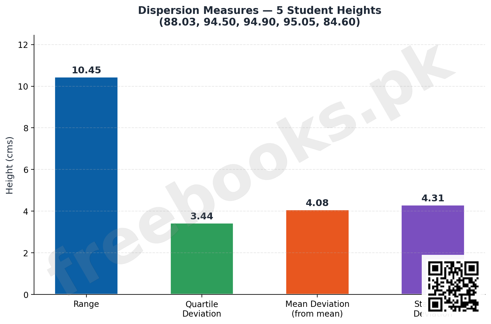
Dispersion Measures Compared: Range, Quartile Deviation, Mean Deviation (from mean), and Standard Deviation calculated for the same 5-value student height data used throughout this chapter's worked examples, shown side by side as a bar chart
Mesokurtic, Platykurtic and Leptokurtic Distributions: Three distribution curves with equal variance illustrating kurtosis: mesokurtic (normal peak), leptokurtic (sharper peak, heavier tails), and platykurtic (flatter peak, lighter tails)
Short Questions & Answers
Why is a measure of central tendency alone insufficient to describe a data set?
Because two data sets can share the exact same mean while having very different amounts of spread, so a single central value hides important information about variability.
What is the key difference between an absolute and a relative measure of dispersion?
An absolute measure keeps the same units as the original data (e.g., cm), while a relative measure is a unit-free ratio, making it useful for comparing variability across data sets measured in different units or scales.
Why can quartile deviation never be negative?
Because the third quartile Q3 is always at least as large as the first quartile Q1, so their difference (and hence Q.D) is always zero or positive.
Why is mean deviation from the median described as the 'smallest possible' mean deviation?
Because the sum of absolute deviations from the median is mathematically smaller than the sum of absolute deviations from any other single value, including the mean.
Why is standard deviation preferred over variance for reporting results?
Because standard deviation is expressed in the original units of the data, while variance is expressed in squared units, which are harder to interpret directly.
Why is the coefficient of variation useful when comparing two data sets with very different means?
Because it expresses variability as a percentage of the mean, allowing fair comparison between groups whose means (and possibly units) differ substantially.
What does it mean if root-beta-1 is negative?
It indicates the distribution is negatively skewed, meaning it has a longer tail extending toward smaller values.
How does a leptokurtic distribution differ visually from a platykurtic one?
A leptokurtic distribution is more sharply peaked with heavier tails, while a platykurtic distribution is flatter, with more values spread between the centre and the tails.
Long Questions & Answers
Explain range, quartile deviation, mean deviation, and standard deviation as measures of dispersion, comparing their merits and demerits.
What is the range, and what are its strengths and weaknesses as a measure of dispersion?
The range is the simplest measure of dispersion: the difference between the largest and smallest observation in a data set. Its great virtue is ease of calculation, requiring only that the two extreme values be identified, making it a genuinely useful quick check, particularly for small samples. Its weakness is severe: because it depends on only two values, it completely ignores everything in between, and it is extremely sensitive to a single unusually large or small observation, which can inflate the range without reflecting the typical spread of the bulk of the data.
What is quartile deviation, and how does it improve on the range?
Quartile deviation looks at the middle half of the data instead of the two most extreme points: it is defined as half the difference between the third quartile and the first quartile. Because it excludes the most extreme twenty-five percent of values on either end, it is far less sensitive to outliers than the range, and is still reasonably easy to calculate once the quartiles are known. Its weakness is that, like the range, it is not based on all observations — two data sets sharing the same quartiles report identical quartile deviations even if their remaining values differ substantially.
What is mean deviation, and what is its main weakness?
Mean deviation is the first of these measures to incorporate every single observation: it is calculated as the average of the absolute deviations of every observation from a chosen central value, typically the mean or median, with 'absolute' meaning every deviation is treated as a positive distance regardless of direction. This makes it considerably more representative of the whole data set than the range or quartile deviation. Its weakness is mathematical: forcing every deviation to be positive through the absolute value operation makes mean deviation very difficult to use in further algebraic development.
What is standard deviation, and how does it solve mean deviation's weakness?
Standard deviation solves mean deviation's mathematical problem by squaring the deviations instead of taking their absolute value. Squaring, like absolute value, guarantees a positive result, but unlike absolute value it is a smooth, well-behaved operation that supports extensive further mathematical development, which is why standard deviation (and the variance that precedes it) underlies most advanced statistical techniques. Standard deviation is based on all observations, like mean deviation, but is more mathematically tractable, at the cost of a two-step process: squaring deviations to get variance, then taking a square root to return to the original units.
Explain the coefficient of variation, why it is needed in addition to standard deviation, and describe how skewness and kurtosis extend the description of a distribution beyond location and spread.
Why is the coefficient of variation needed in addition to standard deviation?
Standard deviation is expressed in the same units as the original data, so it cannot be used directly to compare variability between data sets measured in different units, or even the same units but very different magnitudes. For instance, a standard deviation of five kilograms represents enormous relative variability among newborn baby weights averaging around three kilograms, but the same five kilograms represents barely any relative variability among adult body weights averaging around seventy kilograms. The raw number alone does not carry enough context to judge whether the spread is large or small relative to the data.
How is the coefficient of variation calculated and interpreted?
The coefficient of variation expresses the standard deviation as a percentage of the mean: C.V equals the standard deviation divided by the mean, multiplied by one hundred. Because this divides one quantity by another measured in the same units, the units cancel out, leaving a dimensionless percentage that can be compared meaningfully across data sets regardless of their original units or scales. A lower coefficient of variation indicates a comparatively more consistent data set, with spread small relative to its own average, while a higher coefficient indicates comparatively more variability relative to the average.
What is skewness, and how do numerical skewness coefficients work?
Skewness measures the lack of symmetry in a distribution. A perfectly symmetrical distribution has its mean, median, and mode all coinciding at the same central point, with the frequency curve on one side a mirror image of the other. A skewed distribution has one tail stretched noticeably longer, either toward larger values (positive skew) or smaller values (negative skew). Numerical measures, such as Karl Pearson's coefficients or Bowley's quartile-based coefficient, condense this shape into a single number: zero for symmetry, negative for a longer left tail, and positive for a longer right tail.
What is kurtosis, and what are leptokurtic and platykurtic distributions?
Kurtosis describes how sharply peaked a distribution is around its centre and how heavy or light its tails are, relative to the standard, moderately-peaked mesokurtic (normal) shape. A leptokurtic distribution is more sharply peaked than normal, with many observations clustered tightly around the mean but also, somewhat counterintuitively, an unusually large number of observations out in the extreme tails. A platykurtic distribution is comparatively flatter than normal, with observations more evenly spread between the centre and the tails rather than concentrated in either region.
Multiple Choice Questions (MCQs)
Which of the following is a relative (unit-free) measure of dispersion? (A) Range (B) Standard deviation (C) Coefficient of variation (D) Variance
Correct answer: (C) Coefficient of variation. The coefficient of variation is a ratio (S / mean x 100) and is therefore unit-free; the others carry the original units.
Quartile deviation is calculated as: (A) Q3 – Q1 (B) (Q3 – Q1) / 2 (C) (Q3 + Q1) / 2 (D) Q3 x Q1
Correct answer: (B) (Q3 – Q1) / 2. Quartile deviation (semi-interquartile range) is Q.D = (Q3 – Q1) / 2.
Mean deviation is smallest when calculated from: (A) The mean (B) The mode (C) The median (D) The range
Correct answer: (C) The median. Mean deviation from the median is always less than or equal to mean deviation from any other value.
Standard deviation is: (A) The mean of squared deviations (B) The positive square root of variance (C) The same as mean deviation (D) Always negative
Correct answer: (B) The positive square root of variance. Standard deviation is defined as the positive square root of the variance.
If every observation in a data set is multiplied by a constant a, the variance is multiplied by: (A) a (B) a^2 (C) 2a (D) 1/a
Correct answer: (B) a^2. Variance scales by the square of the constant: var(aY) = a^2 * var(Y).
The coefficient of variation is useful because it: (A) Has the same units as the data (B) Is always equal to zero (C) Is unit-free and allows comparison across data sets (D) Cannot be expressed as a percentage
Correct answer: (C) Is unit-free and allows comparison across data sets. C.V is a dimensionless ratio expressed as a percentage, making it ideal for comparing variability across different units or scales.
The second moment about the mean (m2) is identical to: (A) The range (B) The variance (C) The mode (D) The coefficient of variation
Correct answer: (B) The variance. The second central moment m2 equals the variance S^2.
A positively skewed distribution has: (A) A longer tail to the left (B) A longer tail to the right (C) No tail at all (D) Mean equal to mode
Correct answer: (B) A longer tail to the right. A positively skewed distribution has a longer tail extending to the right-hand side.
Bowley's coefficient of skewness is based on: (A) Mean and mode only (B) Range only (C) Quartiles and the median (D) Standard deviation only
Correct answer: (C) Quartiles and the median. Bowley's coefficient uses (Q1 + Q3 – 2*Median) / (Q3 – Q1).
A leptokurtic distribution compared to a mesokurtic (normal) one is: (A) Flatter with lighter tails (B) More sharply peaked with heavier tails (C) Identical in shape (D) Always negatively skewed
Correct answer: (B) More sharply peaked with heavier tails. Leptokurtic distributions are more peaked with heavier tails than the normal (mesokurtic) shape.
Quick Revision Summary
- Absolute measures (same units as data): Range, Q.D, M.D, Variance, S.D. Relative measures (unit-free): C.V and coefficients of dispersion
- Range R = Y(n) – Y(1); simple but ignores all but the two extreme values
- Quartile deviation Q.D = (Q3 – Q1)/2; not affected by extremes but ignores most of the data
- Mean deviation M.D = mean of |Y – M|; based on all values but hard to develop mathematically
- Variance = mean of squared deviations from mean; S.D = positive square root of variance
- Variance is unaffected by adding a constant (change of origin); scales by a^2 under multiplication (change of scale)
- Coefficient of variation C.V = (S / mean) x 100; unit-free, ideal for comparing different data sets
- Moments: m1=0 always, m2=variance, m3 relates to skewness, m4 relates to kurtosis
- Skewness: zero=symmetric, negative=left tail longer, positive=right tail longer
- Kurtosis: mesokurtic=normal peak, leptokurtic=more peaked/heavier tails, platykurtic=flatter
Exam Tips
- When a question asks to 'compare variability' between two data sets with different units or means, that's a signal to use coefficient of variation, not raw standard deviation
- Remember the short-cut variance formula S^2 = (sum Y^2)/n – (mean)^2 — much faster than computing every deviation by hand
- Quartile deviation and mean deviation both ignore the sign of spread (never negative) — only variance/S.D. use squaring to achieve this
- For grouped data with equal class width, use the coding variable u=(y-a)/h to simplify moment calculations before converting back
- Remember: variance is unaffected by shifting all data by a constant, but scales by the square of any multiplier
- Bowley's coefficient of skewness only needs Q1, Q2 (median), and Q3 — no need to calculate the mean at all