Statistics Class 11 Chapter 3 Notes – Measures of Location (ICS Part-I)

A diagram or a frequency table gives an overall impression of a data set, but it does not give a single number that tells us where the 'centre' of the data lies. This chapter covers the measures used for exactly that purpose: arithmetic mean, weighted mean, geometric mean, harmonic mean, median and mode. These are collectively called averages, measures of location, or measures of central tendency, because each one gives an indication of where to locate the distribution on the number line.

Along with the measures of central tendency, this chapter also covers quantiles — quartiles, deciles, and percentiles — which describe the position of a particular observation relative to the rest of the data set, rather than just the centre. The chapter closes with the empirical relationship connecting mean, median and mode for skewed distributions, and guidance on selecting the most suitable measure for a given type of data.

Learning Objectives

• Calculate the arithmetic mean for ungrouped and grouped data, including by the short-cut (coding) method
• Explain and calculate the weighted mean, and identify when it is preferred over the ordinary mean
• Calculate the geometric mean and harmonic mean, and identify situations where each is appropriate
• State and apply the general relationship AM >= GM >= HM
• Calculate the median for ungrouped and grouped (continuous and discrete) data
• Calculate quartiles, deciles, and percentiles for ungrouped and grouped data
• Calculate the mode for ungrouped and grouped data
• State the empirical relationship between mean, median and mode for skewed distributions
• Select an appropriate measure of central tendency for a given situation

Key Concepts

3.1 Introduction

A single quantitative measure is needed to indicate the centre of a distribution. The measures commonly used for this are mean, median and mode, with geometric mean and harmonic mean used in specific situations. A good average should be well defined, easy to calculate, easy to understand, based on all the values, and capable of mathematical treatment. The important types of averages covered in this chapter are: arithmetic mean and weighted mean, geometric mean, harmonic mean, median, and mode.

3.2 Arithmetic Mean and Weighted Mean

The arithmetic mean is calculated by adding up all the observations and dividing the sum by the total number of observations. For a population of N observations it is denoted by the Greek letter mu (a parameter, a fixed but usually unknown value); for a sample of n observations it is denoted by Y-bar (a statistic whose value varies from sample to sample) and is a good, unbiased estimate of the population mean. The arithmetic mean carries the same units as the original observations.

For grouped data, the arithmetic mean is calculated as the sum of (frequency x class midpoint) divided by the sum of frequencies, since each observation in a class is assumed equal to that class's midpoint. This assumption causes a small difference between the mean of grouped data and the mean of the same data left ungrouped, called grouping error. The mean can also be calculated by the short-cut (coding) method: an arbitrary provisional mean 'a' is chosen, deviations D = Y – a are computed, and the true mean is recovered as a plus the average deviation — useful for simplifying arithmetic by hand.

Key properties of the arithmetic mean: the algebraic sum of deviations of observations from their mean is always zero; a combined mean of two or more groups can be calculated from each group's mean and size; the sum of squared deviations from the mean is smaller than the sum of squared deviations from any other value (this is why the mean 'minimizes' squared error); the mean shifts by a constant amount when that constant is added to every observation (change of origin); and the mean scales by a constant factor when every observation is multiplied by that factor (change of scale).

Merits of the arithmetic mean: rigidly defined by a formula, easy to calculate and understand, based on all values, stable across repeated samples, and the total can be recovered if the mean and count are known. Demerits: very sensitive to departures from a bell-shaped distribution (unsuitable for skewed data), can be misleading with high variation, greatly affected by extreme values, and cannot be calculated for open-end classes without assuming their open ends.

The weighted mean is used when different observations should not be given equal importance — each value Yi is given a weight wi, and the weighted mean is the sum of (wi times Yi) divided by the sum of the weights.

3.3 Geometric Mean

The geometric mean (G.M) is defined as the nth root of the product of n positive values, and is appropriate only for positive, ratio-scale data — it is particularly useful for averaging rates, ratios, percentage changes, and index numbers. It is commonly calculated via logarithms: the log of the G.M. equals the average of the logs of the observations, and G.M. is then found by taking the antilog. For grouped data, each value's log is weighted by its class frequency before averaging.

Key properties: a combined geometric mean of several groups can be found from each group's geometric mean and size; and the geometric mean of a ratio of two matched data sets equals the ratio of their individual geometric means. Merits: rigidly defined, based on all observations, capable of further mathematical development, and less affected by extreme values than the arithmetic mean. Demerits: becomes zero if any observation is zero, and is undefined (imaginary) for negative values.

3.4 Harmonic Mean

The harmonic mean (H.M) is defined as the reciprocal of the arithmetic mean of the reciprocals of the values, and is particularly useful for averaging rates and ratios that are expressed 'per unit' of something, such as speed (distance per time) — most notably, average speed over equal distances travelled at different speeds. For grouped data it is calculated as the sum of frequencies divided by the sum of (frequency divided by the value).

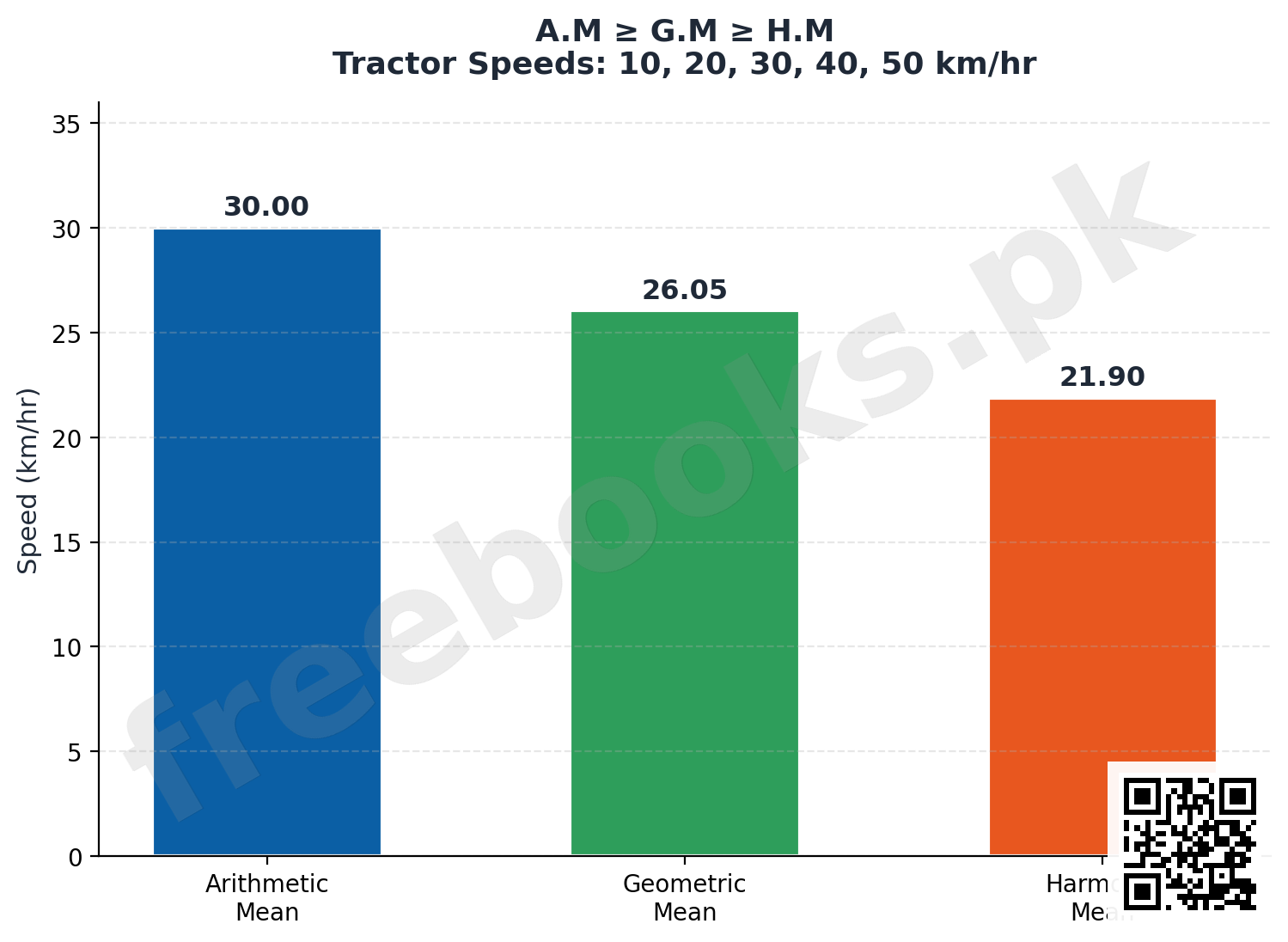
Merits: defined by a formula, based on all observations, capable of further mathematical development. Demerits: cannot be calculated if any observation is zero, more complex to calculate than the arithmetic mean, and gives more relative weight to small values than to large ones. For any set of positive observations, the three means always satisfy AM >= GM >= HM, with equality only when all the observations are identical.

3.5 Median

The median is the value that divides an arranged (ordered) data set into two equal halves. For an odd number of observations n, the median is the value of the ((n+1)/2)th item in the ordered data; for an even number of observations, it is the mean of the (n/2)th and ((n/2)+1)th items. For grouped continuous data, the median is calculated using the formula Median = l + (h/f)(n/2 – c), where l is the lower boundary of the median class, h is its width, f is its frequency, n is the total frequency, and c is the cumulative frequency of the class preceding the median class; the median class itself is located by finding which class contains the (n/2)th observation using the cumulative frequency column. For discrete grouped data, the median is found directly from the formal definition using a cumulative frequency column.

Key properties: adding a constant to every observation shifts the median by that same constant, and multiplying every observation by a constant scales the median by that factor; the sum of absolute deviations from the median is smaller than from any other value; and for a symmetrical distribution, the median is equidistant from the first and third quartiles. Merits: quick to find, not much affected by extreme values, and suitable for skewed distributions. Demerits: not rigidly defined, not readily suitable for further algebraic development, less stable across repeated samples than the mean, and not based on all the observations.

3.6 Quantiles: Quartiles, Deciles and Percentiles

Quantiles (also called fractiles) describe the position of an observation relative to the rest of a data set. Quartiles divide the ordered data into four equal parts: Q1 (lower quartile) exceeds one quarter of the observations, Q2 is the median, and Q3 (upper quartile) exceeds three quarters of the observations. For grouped data, Qk = l + (h/f)(k.n/4 – c) for k = 1, 2, 3, using the same lower-boundary/width/frequency/cumulative-frequency logic as the median formula, just targeting a different fraction of n.

Deciles divide the ordered data into ten equal parts (D1 through D9), with D5 equal to the median; for grouped data, Dm = l + (h/f)(m.n/10 – c). Percentiles describe finer relative standing, dividing the data into 100 parts (P1 through P99); for grouped data, Pm = l + (h/f)(m.n/100 – c). By definition, P50 is the median, P25 is Q1, and P75 is Q3 — quartiles, deciles and percentiles are simply different granularities of the same underlying idea, and can also be read directly off a cumulative frequency (ogive) graph.

3.7 Mode

The mode is the most frequently occurring value in a data set. For ungrouped data, it is found directly by inspecting which value occurs most often. Data with exactly one mode is called unimodal; data can also be bimodal (two modes), multimodal (more than two modes), or have no mode at all if every value occurs equally often. For grouped continuous data, the mode is calculated using Mode = l + (fm – f1)/((fm – f1)+(fm – f2)) x h, where l is the lower boundary of the modal class (the class with the highest frequency), fm is the modal class's frequency, f1 and f2 are the frequencies of the classes immediately before and after the modal class, and h is the modal class width.

Merits of the mode: very quick to find, and not affected by extreme values. Demerits: not rigidly defined, not easily suited to further mathematical development, uses only a few members of the data set (so it can be misleading in small samples), unstable across repeated samples like the median, may have more than one value, and may not exist at all for some data sets.

3.7.4 Empirical Relationship Between Mean, Median and Mode

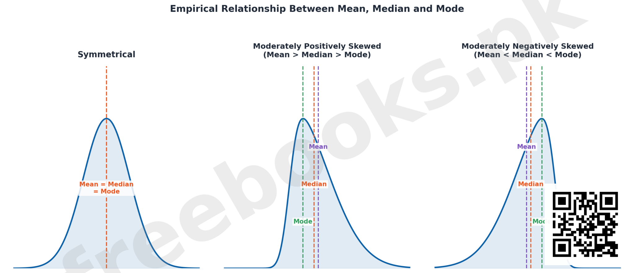
This relationship depends on the shape of the distribution. A distribution is symmetrical if the frequency curve's left side, mirrored about the mean, matches its right side; otherwise it is called skewed (to the right or to the left). For a single-peaked symmetrical distribution, Mean = Median = Mode. For a moderately positively skewed distribution, Mean > Median > Mode. For a moderately negatively skewed distribution, Mean < Median < Mode. For moderately skewed distributions generally, the median divides the distance between the mean and the mode in the ratio 1:2, which gives the useful empirical shortcut: Mode = 3 x Median – 2 x Mean.

3.8 Selecting a Suitable Measure of Central Tendency

Choosing the right measure depends on the type of variable, the purpose of the statistic, and the shape of the distribution. For quantitative variables, the arithmetic mean is usually appropriate. For categorical variables, median or mode is preferred depending on the type of category — for example, mode suits eye colour, while median suits ordered income groups. If a distribution is symmetrical, mean, median and mode are equal and equally good; for skewed distributions, the median is preferred since it is not affected by extreme values, and medians are also preferred over means when the sample is only a small part of the population. Geometric and harmonic means are reserved specifically for averaging rates and ratios.

Important Definitions

Key Facts and Relations

Topic	Key Fact / Relation
Population mean	mu = (sum of Y) / N
Sample mean (grouped data)	Y-bar = (sum of fi * yi) / (sum of fi)
Short-cut (coding) method	Y-bar = a + (sum of fi*Di) / (sum of fi), where Di = Yi – a
Weighted mean	Y-bar(w) = (sum of wi*Yi) / (sum of wi)
Geometric mean (ungrouped)	G.M = (Y1 x Y2 x … x Yn)^(1/n) = antilog[(sum of log Yi)/n]
Harmonic mean (ungrouped)	H.M = n / (sum of 1/Yi)
General relationship	A.M >= G.M >= H.M (equal only if all observations are identical)
Median (grouped data)	Median = l + (h/f)(n/2 – c)
Quartiles (grouped data)	Qk = l + (h/f)(k.n/4 – c), for k = 1, 2, 3
Deciles (grouped data)	Dm = l + (h/f)(m.n/10 – c)
Percentiles (grouped data)	Pm = l + (h/f)(m.n/100 – c)
Mode (grouped data)	Mode = l + [(fm – f1) / ((fm – f1)+(fm – f2))] x h
Empirical relation (skewed data)	Mode = 3 x Median – 2 x Mean

Diagrams

Symmetrical vs. Skewed Distributions: Three frequency curves comparing the relative positions of mean, median and mode: symmetrical (all three equal), moderately positively skewed (Mean > Median > Mode), and moderately negatively skewed (Mean < Median < Mode)

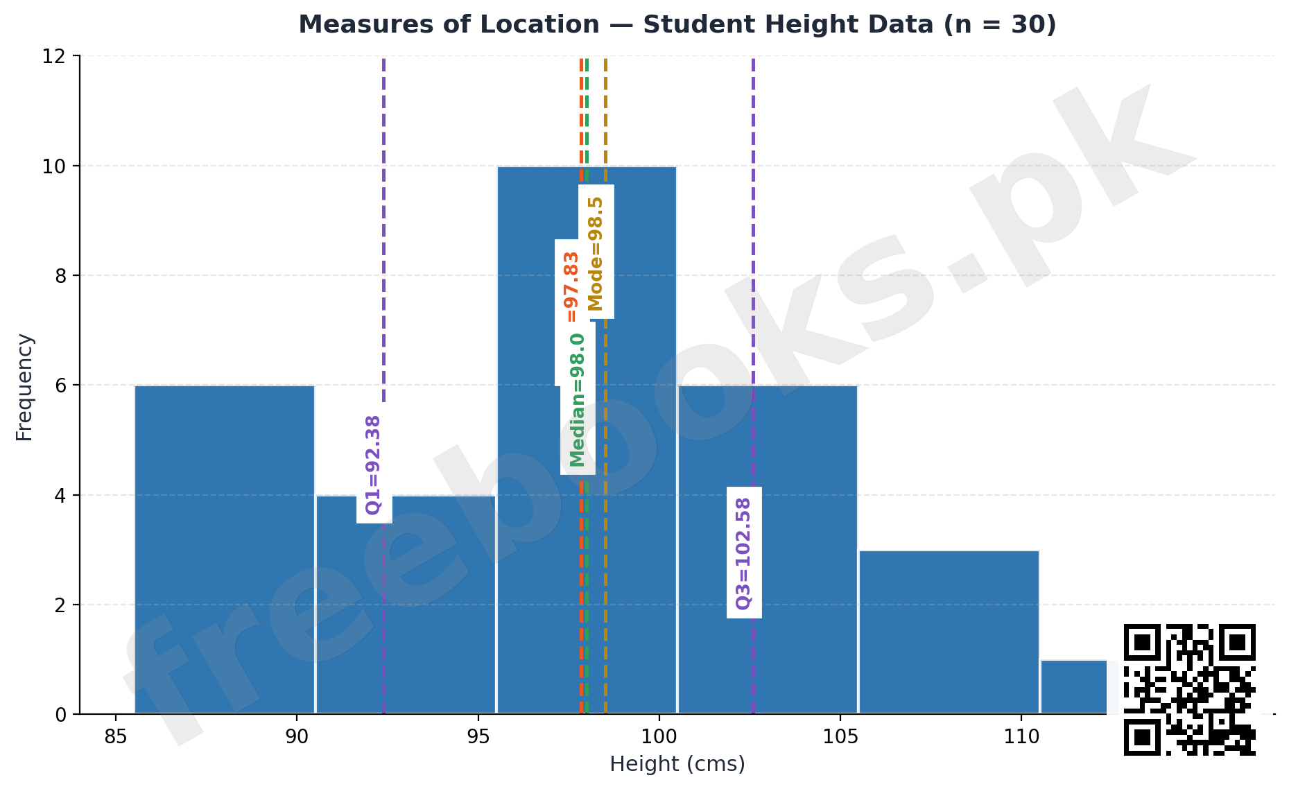
Measures of Location on the Student Height Data: The student-height histogram (from Chapter 2) with the calculated mean, median, and mode marked, alongside Q1 and Q3, showing how these measures locate the centre and spread of the same data set

A.M >= G.M >= H.M for the Tractor Speed Example: A bar comparison of the arithmetic mean, geometric mean, and harmonic mean calculated from the same worked example (tractor speeds of 10, 20, 30, 40, 50 km/hr over equal distances), illustrating the general relationship A.M >= G.M >= H.M

Short Questions & Answers

Long Questions & Answers

Explain the arithmetic mean, geometric mean, and harmonic mean, including when each is the appropriate choice, and state the relationship between them.

What is the arithmetic mean, and how is it calculated for grouped data?

The arithmetic mean is calculated by adding up all observations and dividing by their count. For a population of N observations it is denoted by the Greek letter mu, and for a sample of n observations it is denoted Y-bar, which is a good, unbiased estimate of the unknown population mean. For grouped data, it is calculated as the sum of each class's frequency multiplied by its midpoint, divided by the total frequency, under the assumption that every observation within a class equals that class's midpoint — an assumption that introduces a small grouping error.

When is the arithmetic mean the appropriate choice, and what is its main weakness?

The arithmetic mean is the natural default choice for quantitative data that is roughly symmetrically distributed, since it uses every observation and is easy to calculate and interpret. It is also, however, the measure most distorted by extreme values or a strongly skewed shape, since a few very large or very small values can pull it noticeably away from where most of the data actually lies. This makes it a poor choice whenever a data set contains significant outliers or heavy skew.

What is the geometric mean, and when is it the appropriate choice?

The geometric mean is defined as the nth root of the product of n positive values, and is calculated in practice by averaging the logarithms of the observations and then taking the antilog of that average. Because it works multiplicatively rather than additively, it is the appropriate choice for averaging rates of change, ratios, percentage growth figures, and index numbers, where a doubling and a halving should cancel out. It is only defined for positive values, becoming zero if any observation is zero and undefined if any observation is negative.

What is the harmonic mean, and when is it the appropriate choice?

The harmonic mean is defined as the reciprocal of the arithmetic mean of the reciprocals of the observations. It is the correct choice when averaging rates or ratios expressed 'per unit' of some other varying quantity, the classic example being average speed, where a vehicle covers equal distances at different speeds. Naively averaging the speeds with the arithmetic mean gives a misleadingly high answer, because it fails to account for more time being spent travelling at the slower speeds. Like the geometric mean, the harmonic mean is undefined if any observation is zero.

What is the relationship between the arithmetic, geometric, and harmonic means?

For any set of positive observations that are not all identical, these three means always satisfy the ordering A.M is greater than or equal to G.M, which is in turn greater than or equal to H.M. The three become exactly equal only when every observation in the data set is the same value. This ordering is a general mathematical fact holding regardless of what the data represents, and it explains why choosing the wrong type of mean for a given kind of data will systematically produce an inflated answer.

Describe how the median, quartiles, deciles and percentiles are calculated for grouped data, and explain what each of these measures tells us about a data set.

What do the median, quartiles, deciles, and percentiles have in common, and how is the median calculated for grouped data?

The median, quartiles, deciles, and percentiles are all members of the same family of measures, called quantiles or fractiles, sharing the idea of identifying positions that split an ordered data set into equal-sized groups rather than summarizing it with one 'typical' value like the mean. The median splits an ordered data set exactly in half. For grouped, continuous data, it is calculated as Median = lower boundary of the median class + (class width / class frequency) x (n/2 – cumulative frequency before that class), where the median class is located by finding which class contains the n/2th observation.

How are quartiles calculated for grouped data?

Quartiles divide the data into four equal parts: the first quartile Q1 is the value below which one quarter of observations fall, the second quartile Q2 is the median itself, and the third quartile Q3 is the value below which three quarters of observations fall. For grouped data, each quartile uses essentially the same formula as the median, except the targeted fraction of the total frequency changes — one quarter of n for Q1, half of n for Q2, and three quarters of n for Q3 — with the appropriate class boundary, width, frequency, and preceding cumulative frequency substituted in.

What are deciles, and how are they calculated?

Deciles carry the same idea of subdivision further, splitting the ordered data into ten equal parts denoted D1 through D9, with the fifth decile D5 always identical to the median. The formula follows the same pattern used for the median and quartiles, this time targeting m tenths of the total frequency for the mth decile, with the corresponding class boundary, width, frequency, and preceding cumulative frequency substituted in for that target. Like quartiles, deciles describe where a value or class stands relative to the whole ordered data set.

What are percentiles, and which quantiles coincide with which percentiles?

Percentiles go furthest of all, dividing the data into one hundred equal parts denoted P1 through P99. By definition, several named quantiles coincide exactly: the 50th percentile P50 is the median, the 25th percentile P25 is the first quartile Q1, and the 75th percentile P75 is the third quartile Q3. Like the median, quartiles, and deciles, percentiles are calculated for grouped data using the same underlying formula, targeting whatever fraction of the total frequency corresponds to the desired percentile.

What do quantiles reveal that a simple average cannot, and how can they be read from a graph?

Quantiles give a sense of relative standing — where a value or class sits relative to the rest of the data, rather than just the overall centre. For example, knowing a student's height falls at the 90th percentile immediately conveys that the student is taller than roughly ninety percent of peers, a far more specific statement than simply knowing the average height. As a practical convenience, all these quantiles can be read directly off a cumulative frequency graph (an ogive) without applying the formula, by locating the desired cumulative frequency on the vertical axis and reading across.

Multiple Choice Questions (MCQs)

Quick Revision Summary

• Arithmetic mean = sum of values / count; sensitive to extreme values and skew
• Weighted mean used when observations carry different importance (weights wi)
• Geometric mean: nth root of product of positive values; best for rates, ratios, percentage changes
• Harmonic mean: reciprocal of mean of reciprocals; best for speeds/rates over equal distances
• General relation: A.M >= G.M >= H.M (equal only if all values identical)
• Median splits ordered data in half: middle value (odd n) or mean of two middle values (even n)
• Grouped-data formulas (median, quartiles, deciles, percentiles) all use: l + (h/f)(target – c)
• Quartiles (4 parts), Deciles (10 parts), Percentiles (100 parts) — P50=Median=Q2, P25=Q1, P75=Q3
• Mode = most frequent value; grouped mode formula uses fm, f1 (preceding), f2 (following)
• Empirical relation for skewed data: Mode = 3 Median – 2 Mean

Exam Tips

• Memorize the grouped-data pattern l + (h/f)(target – c) — it's identical for median, quartiles, deciles, and percentiles, only the target fraction of n changes
• For AM/GM/HM word problems, identify whether the question involves rates (HM), ratios/growth (GM), or plain totals (AM) before choosing a formula
• Always order the data first before finding median, quartiles, or percentiles by the direct/formal definition
• Remember P50 = Median = Q2 and P25 = Q1, P75 = Q3 — these equivalences are common exam questions
• For the empirical relation, remember the ratio is 1:2 (mean-median gap : median-mode gap), giving Mode = 3 Median – 2 Mean
• Mode can fail to exist or have multiple values — always check ungrouped data by inspection first