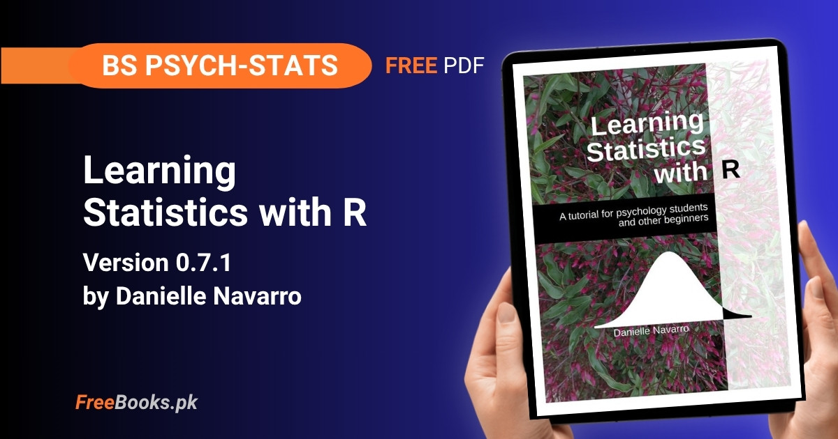
Learning Statistics with R is a free textbook by Danielle Navarro that teaches an introductory statistics course through the R language, written for students who want to understand the ideas rather than memorise formulas. It began as lecture notes for an undergraduate psychology class and grew into a 17-chapter, 796-page book covering research design, R basics, descriptive statistics, probability, estimation, hypothesis testing, chi-square tests, t-tests, ANOVA, regression and a closing chapter on Bayesian statistics.
For BS Psychology and BS Statistics students, it works as a first-course companion and as a revision guide. Every test is built up from the logic behind it and then run in R, so you can check a hand calculation against software output. This edition is a faithful Quarto port of the original book, released under CC BY-SA 4.0. The statistics have held up well, while the R code is older base-R style, and this page says plainly where that matters.
Book Overview
| Course | Statistics with R (introductory applied statistics) |
| Degree Programs | BS Psychology, BS Statistics |
| Level | Undergraduate, introductory (no prior statistics or R assumed) |
| Edition | Version 0.7.1 (Quarto edition), changelog dated 7 October 2026 |
| Author | Danielle Navarro |
| Publisher | Self-published by the author (no commercial publisher) |
| Structure | 6 parts, 17 chapters plus an Epilogue, and a Data sets page listing every file used (796 pages in the PDF) |
| Exercises | No end-of-chapter exercise sets; learning is through worked R examples on the data sets |
| Language | English |
| License | Creative Commons Attribution-ShareAlike 4.0 (CC BY-SA 4.0) — Model: Link-only |
| Format | Free PDF and free HTML edition on the author’s website |
Chapter List
Chapter 1: Why Do We Learn Statistics?
Part I: Background · Difficulty: Easy · Key topics: statistics as a safeguard, belief bias, Simpson’s paradox, aggregated vs. disaggregated data, base rates, statistics in psychology
The opening chapter asks why scientists run statistics instead of trusting common sense, and answers that we do not trust our own judgement: gut instinct and verbal argument are open to bias, and the belief bias effect shows people judging an argument by how believable its conclusion sounds. It then tells the 1973 Berkeley admissions story. Overall, 44% of male applicants but only 35% of female applicants were admitted, yet within each department the pattern leans slightly the other way. That is Simpson’s paradox. The chapter closes on why psychology is so statistical and on common errors in news reports.
Key Points:
- Statistics is a safeguard against our own biases, not a replacement for careful thought
Belief bias: people judge whether an argument is logically valid by whether its conclusion sounds believableSimpson's paradox: a pattern in combined data can reverse or vanish once the data are split into subgroups- In the Berkeley data, the overall admission gap came from which departments men and women applied to, not from bias inside each department
- Whether to analyse aggregated or disaggregated data depends on the question you are asking, and statistics alone cannot decide that
- A percentage reported without a baseline for comparison is one of the most common statistical errors in news stories
Memory Tip: Whenever a group-level number surprises you, ask what is hiding inside it: split by the obvious third variable and see if the story survives.
Common Mistake: Treating a headline percentage as proof of bias or of an effect without checking the subgroups it is built from.
Important Questions:
- What is Simpson’s paradox? A trend that appears in aggregated data but reverses or disappears when the data are broken into subgroups; the Berkeley admissions data are the book’s example.
- Why do scientists use statistics instead of common sense? Because intuition and verbal reasoning are open to bias (belief bias is one documented case), and statistics gives a disciplined check on our own judgement.
Chapter 2: A Brief Introduction to Research Design
Part I: Background · Difficulty: Easy · Key topics: operationalisation, scales of measurement, reliability, predictors and outcomes, experimental vs. non-experimental research, types of validity, threats to validity, replication crisis
This chapter treats data collection as measurement. It starts with operationalising a theoretical construct, then covers the four scales of measurement and the continuous/discrete split. Reliability comes next (test-retest, inter-rater, parallel forms, internal consistency), followed by the predictor/outcome vocabulary and the difference between experiments, where the researcher manipulates the predictor and randomises, and non-experimental studies. The long second half lists the kinds of validity and a catalogue of threats: history, maturation, selection bias, attrition, regression to the mean, experimenter and demand effects, and placebo effects. It ends with fraud and the reform movement after the replication crisis.
Key Points:
Operationalisationturns a theoretical idea such as “anxiety” into something you can actually measure- Four scales:
nominal(labels),ordinal(order only),interval(equal steps, no true zero),ratio(true zero) - Reliability is repeatability, validity is whether you measure the right thing; a measure can be reliable and still invalid
- In an experiment the researcher manipulates the predictor (IV) and uses random assignment so groups differ only by chance
- Validity comes in internal, external, construct, face and ecological forms
Regression to the mean: units picked for an extreme score tend to score less extremely next time, purely by chance
Memory Tip: Reliability asks “do I get the same answer every time?” and validity asks “is it the right answer?”; a bathroom scale can be perfectly reliable even when you are holding a sack of potatoes.
Common Mistake: Assuming a measure is valid just because it gives consistent results, or that an effect is caused by the treatment when the groups were never randomly assigned.
Important Questions:
- What is the difference between reliability and validity? Reliability is the consistency of a measurement; validity is whether it measures what you intend it to measure.
- What makes a study an experiment rather than non-experimental research? The researcher controls the study and manipulates the predictor variable, normally with random assignment, so that a causal effect on the outcome can be assessed.
Chapter 3: Getting Started with R
Part II: An Introduction to R · Difficulty: Easy · Key topics: installing R, RStudio and Positron, the console, arithmetic, variables and assignment, functions and arguments, vectors, logical values, indexing
Chapter 3 contains no statistics on purpose; the goal is to get comfortable typing commands. It argues for doing statistics in R rather than in a spreadsheet or proprietary package, then covers installing R and an IDE (RStudio or Positron). From there you use the console as a calculator, store values in variables with the assignment arrow, call functions with named arguments and defaults, and build vectors with c(). The chapter introduces numeric, text and logical data, the logical operators, and logical indexing for pulling elements out of a vector.
Key Points:
- Assign a value with
x <- 5; variable names are case sensitive, soSalesandsalesdiffer - Arithmetic operators are
+ - * / ^, and R follows the usual order of operations - Functions such as
sqrt(),abs(),round(),nchar()andlength()take arguments that can be named and often have defaults c()combines values into a vector; indexing with square brackets extracts elements- Three basic data types: numeric, character (text) and logical (
TRUE/FALSE) - Logical operators:
== != < > <= >= ! & |, and logical vectors can be used as indexes
Practice Tip: Type each example yourself instead of pasting it; a mistyped command produces an error message, and learning to read those messages is half the skill.
Common Mistake: Using a single = when you meant the comparison ==, or forgetting that capitalisation matters in names.
Important Questions:
- How do you store a number in a variable in R? Use the assignment operator, for example
x <- 10, and then usexin later calculations. - What does logical indexing do? It uses a vector of
TRUE/FALSEvalues (for example the result ofx > 5) to select only the elements for which the condition holds.
Chapter 4: R Mechanics
Part II: An Introduction to R · Difficulty: Easy · Key topics: comments, packages, workspace, file system, loading and saving data, special values, factors, data frames, lists, formulas, generic functions, help files
This chapter fills in the practical machinery you need before real analysis. The first half covers comments, installing and loading packages, keeping the workspace tidy, navigating the file system, and loading and saving data, including CSV files. The second half moves to the kinds of variable you will meet: special values such as NA, element names, classes, factors for categorical data, data frames for a whole data set, lists and formulas. It finishes with generic functions, which explain why one function can behave differently on different objects, and with how to read R’s help pages.
Key Points:
- A package is installed once with
install.packages()and loaded in each session withlibrary() - The workspace holds your variables;
objects()orwho()(from the lsr package) lists them andrm()removes them - The working directory decides where R looks for files;
load()reads workspace files andread.csv()imports CSV files - A
factorstores categorical data as labelled levels; adata framestores variables as columns, accessed with$ - A formula such as
outcome ~ predictordescribes a relationship and is used by many modelling functions later in the book ?functionopens a help page;??topicsearches the help system
Practice Tip: Load a small CSV file with read.csv(), then run names() or who(TRUE) to see the variables; checking that each column has the class you expect saves many confusing errors later.
Common Mistake: Forgetting to set the working directory (or give the correct path) and then wondering why R cannot find the data file.
Important Questions:
- What is the difference between installing and loading a package? Installing downloads the package to your computer once; loading it with
library()makes its functions available in the current session. - What is a data frame, and how do you pull out one variable? A data frame is a table in which each column is a variable; you extract a column with
$, as indf$score.
Chapter 5: Descriptive Statistics
Part III: Working with Data · Difficulty: Easy · Key topics: mean, median, mode, trimmed mean, range, IQR, variance, standard deviation, skew and kurtosis, standard scores, correlation, missing values
Chapter 5 shows how to summarise a data set compactly, starting from real Australian football margins. It separates central tendency (mean, median, trimmed mean, mode) from variability (range, interquartile range, mean absolute deviation, variance, standard deviation, median absolute deviation) and explains why the mean and median can disagree, using a news example about housing affordability. Skew and kurtosis follow, then R summaries for a variable, a data frame, and each group. The last sections cover z-scores, Pearson and Spearman correlation with their interpretation, and handling missing values.
Key Points:
- The mean is pulled toward extreme values; the median is resistant, so skewed data usually call for the median
- Sample variance divides by
N - 1rather thanN, which is what R’svar()andsd()do Standard deviationis the square root of the variance and is in the same units as the data- A
z-scoreis(X - mean) / sd, how many standard deviations a value sits from the mean - The correlation
rruns from -1 to +1; Spearman’s version uses ranks and suits ordinal or non-linear monotonic data - Always plot the data before interpreting a correlation, as Anscombe’s Quartet shows
Practice Tip: Compute mean() and median() of a skewed variable, then change one value to something extreme and re-run both; seeing only the mean jump makes the difference stick.
Common Mistake: Reporting a single correlation or mean without looking at the data’s shape, when very different data sets can share the same summary numbers.
Important Questions:
- When should you prefer the median to the mean? When the distribution is skewed or has outliers, because the median is not pulled by extreme values the way the mean is.
- Why does R divide by N – 1 when computing variance? A sample tends to understate the population’s spread, so dividing by N – 1 gives a better estimate of the population variance than the plain average of squared deviations.
Chapter 6: Drawing Graphs
Part III: Working with Data · Difficulty: Easy · Key topics: R graphics devices, plot customisation, histograms, stem and leaf plots, boxplots, scatterplots, bar graphs, par(), saving figures, ggplot2
Chapter 6 teaches R’s traditional base graphics through the painter’s model: each command paints onto a device, and you cannot undo a stroke, only start again. It begins with a first plot and how to customise titles, axis labels, plot types and axes, then covers the standard statistical graphs one by one: histograms, stem and leaf plots, boxplots (including multiple boxplots and outlier detection), scatterplots and bar graphs. It ends with global settings through par() and saving image files. A newer epilogue notes that ggplot2 has since become the default choice for most R users.
Key Points:
- R graphics follow the painter’s model: each call adds to the current plot, and mistakes mean redrawing
- A
histogramshows the shape of one numeric variable; bin choices change how it looks - A
boxplotmarks the median, the box covers the middle half (the IQR), and by default whiskers stop at 1.5 times the IQR - Points beyond the whiskers are plotted separately and flagged as possible outliers
- A
scatterplotshows the relationship between two numeric variables, and a bar graph shows counts or summaries for categories par()changes global graphical settings, and figures can be exported to image files
Practice Tip: Draw a histogram of one variable, then change the number of bins or breaks and redraw it; you will see how the same data can look smooth or jagged depending on that single choice.
Common Mistake: Treating the boxplot’s outlier dots as errors to delete, when they are only points beyond the 1.5 x IQR rule and may be perfectly genuine observations.
Important Questions:
- How does R decide where a boxplot’s whiskers end? By default they extend to the most extreme data points within 1.5 times the interquartile range of the box; points beyond that are drawn individually.
- Which graph would you use for the relationship between two numeric variables? A scatterplot, because it shows direction, strength and unusual points before you calculate a correlation.
Chapter 7: Pragmatic Matters
Part III: Working with Data · Difficulty: Medium · Key topics: tabulating, recoding variables, subsetting, sorting and merging, wide vs. long form, text handling, reading unusual files, type coercion, matrices, dates, floating point, recycling
The author calls this chapter a grab bag, a more honest account of how messy real data are. It covers tabulating and cross-tabulating, recoding and transforming variables, and cutting a numeric variable into categories. It then shows how to extract subsets of vectors and data frames, sort, flip and merge data, and reshape between wide and long form. Later sections handle text manipulation, reading SPSS, Excel and other file types, coercing data between classes, matrices, ordered factors and dates, and quirks such as floating point error and the recycling rule. A newer epilogue points to the tidyverse.
Key Points:
table()builds frequency tables from vectors or data frames, and counts can be converted to proportions- A subset can be taken with
subset()or with square brackets[rows, columns]; negative indices drop elements - Repeated-measures data come in wide form (one row per person) or long form (one row per observation), and analyses often need one or the other
- Text tools include shortening, pasting, splitting, converting case and matching or substituting patterns
- Floating point arithmetic is not exact, so comparing decimals with
==can fail - The recycling rule repeats a shorter vector to match a longer one, which can silently hide mistakes
Practice Tip: Take a tiny data frame, sort it by one column, then extract only the rows that meet a condition; doing it two ways (subset() and brackets) shows they give the same result.
Common Mistake: Forgetting the comma inside df[rows, columns], which makes R return a different object than you intended.
Important Questions:
- What is the difference between wide form and long form data? In wide form each participant occupies one row with a column per measurement; in long form each measurement gets its own row, with a variable that records which condition it belongs to.
- Why can
0.1 + 0.2 == 0.3be FALSE in R? Computers store decimals approximately, so tiny rounding errors appear; the chapter’s floating point section explains why exact comparison of decimals is unreliable.
Chapter 8: Basic Programming
Part III: Working with Data · Difficulty: Medium · Key topics: scripts, while and for loops, conditional statements, writing functions, implicit loops
This chapter makes the point that programming is only writing instructions a computer can follow, and that you already have the beginner skills. It starts with scripts, saved files of R commands you can edit and re-run, then covers loops (the while loop, the for loop and a more realistic loop example), conditional statements built from if and else, and writing your own functions with arguments and a returned value. It closes with implicit loops such as sapply() and tapply(), which apply a function across items or groups without writing the loop yourself.
Key Points:
- A script is a text file of R commands; editing and re-running it beats retyping at the console
- A
forloop repeats a block for each value in a vector; awhileloop repeats as long as a condition stays true if (CONDITION) { ... } else { ... }lets a program choose between actions- A function is created with
function(...), runs in its own temporary environment and returns a value sapply()applies a function to each element;tapply()andby()apply one to each group of a grouping variable
Practice Tip: Write a small function (for example one that multiplies its input by four), then call it inside sapply() on a vector; you will see how a loop and a function combine.
Common Mistake: Writing a while loop whose condition never becomes false, so R keeps running until you stop it.
Important Questions:
- What is the difference between a for loop and a while loop? A for loop runs once for each value in a given set; a while loop keeps running until its condition is no longer true.
- What does
tapply()do? It splits a variable by a grouping variable and applies a function, such as the mean, to each group.
Chapter 9: Introduction to Probability
Part IV: Statistical Theory · Difficulty: Medium · Key topics: probability vs. statistics, frequentist and Bayesian views, probability rules, binomial distribution, normal distribution, probability density, t, chi-square and F distributions
Part IV opens with a short essay on the riddle of induction, stressing that statistical inference always rests on assumptions. Chapter 9 itself separates probability, where the model is known and the data are not, from statistics, which works the other way round. It contrasts the frequentist view of probability as long-run frequency with the Bayesian view as degree of belief, sets out the basic rules with elementary events and probability distributions, and then works through the binomial and normal distributions, including the idea of probability density. The t, chi-square and F distributions are previewed with pictures only.
Key Points:
- Probabilities are numbers from 0 to 1, and the probabilities of all elementary events add to 1
- Probability starts from a known model and asks about data; statistics starts from data and asks about the model
- Frequentists define probability as long-run frequency, Bayesians as degree of belief
Binomialdistribution: the number of successes inNindependent yes/no trials, each with the same success probability- The
normaldistribution is a symmetric bell curve described by its mean and standard deviation, and R givesdnorm(),pnorm(),qnorm()andrnorm() - For a continuous variable, density is not probability; probability is the area under the curve over an interval
Memory Tip: Remember the four function prefixes in R: d for density, p for the probability up to a point, q for the quantile, r for random draws.
Common Mistake: Reading the height of a normal curve at a point as the probability of that exact value, when a continuous variable only has probability over intervals.
Important Questions:
- How are probability and statistics different? Probability reasons from a known model to the likely data; statistics reasons from observed data back to the unknown truth about the world.
- When does a binomial distribution apply? When you count successes across a fixed number of independent trials that each have the same probability of success, such as coin flips.
Chapter 10: Estimating Unknown Quantities from a Sample
Part IV: Statistical Theory · Difficulty: Hard · Key topics: populations and samples, simple random sampling, parameters vs. statistics, law of large numbers, sampling distribution, central limit theorem, estimators, standard error, confidence intervals
This chapter introduces the first big idea of inference, estimation, but builds sampling theory first. It defines populations, samples and simple random samples, asks how much it matters when sampling is not random, and distinguishes population parameters from sample statistics. The law of large numbers and the sampling distribution of the mean lead to the central limit theorem. With that in place, it shows how to estimate the population mean and standard deviation and why the standard deviation estimate needs a correction, then builds confidence intervals and discusses their correct interpretation.
Key Points:
- A
parameterdescribes the population; astatisticdescribes the sample you actually have Law of large numbers: as the sample grows, the sample mean settles near the population mean- The standard error of the mean is
sigma / sqrt(N), so it shrinks as the sample grows Central limit theorem: sample means are approximately normally distributed, whatever shape the population has- The sample mean is a good estimate of the population mean, but the sample standard deviation is slightly biased, so divide by
N - 1 - A 95% confidence interval is built around the estimate; it is not a 95% probability that the parameter lies inside this particular interval
Memory Tip: Think of a confidence interval as describing the method, not the one interval: if you repeated the study many times, about 95% of intervals built this way would capture the true value.
Common Mistake: Saying “there is a 95% chance the true mean is inside my interval”, which is the Bayesian reading, not what a frequentist confidence interval means.
Important Questions:
- What does the central limit theorem say? The sampling distribution of the mean becomes approximately normal as the sample size grows, with a spread (the standard error) that shrinks as N increases.
- Why is the population standard deviation estimated with N – 1? The sample standard deviation underestimates the population value, so the N – 1 version corrects that bias.
Chapter 11: Hypothesis Testing
Part IV: Statistical Theory · Difficulty: Hard · Key topics: null and alternative hypotheses, Type I and Type II errors, test statistics, critical regions, p-values, reporting results, effect size, power, Neyman vs. Fisher, p-value debates
Chapter 11 explains how a hypothesis test is built, using a running example of a test for clairvoyance in which 62 of 100 people guess a hidden card correctly. It separates research hypotheses from statistical ones, introduces Type I and Type II errors through a courtroom analogy, and builds a test statistic with its sampling distribution, critical regions and one- or two-sided tests. The p-value comes next, then how to report results, effect size, sample size and power. It closes with the Neyman versus Fisher split, frequentists versus Bayesians, practical traps, and a newer epilogue on life beyond p < .05.
Key Points:
- The null hypothesis
H0is what you try to reject; the alternativeH1is what you accept if you reject it - A
Type Ierror rejects a true null; aType IIerror keeps a false null - The significance level
alpha(commonly .05) is the Type I error rate you are willing to accept - The
p-valueis the probability of getting a result at least this extreme if the null were true - Power is the probability of correctly rejecting a false null; it rises with larger effect size and sample size
- Comparing two groups to chance separately is not the same as testing the difference between them
Memory Tip: Think of a criminal trial: the null is “innocent until proven guilty”, a Type I error convicts an innocent person, and a Type II error lets a guilty person go free.
Common Mistake: Reading the p-value as the probability that the null hypothesis is true, or treating “not significant” as proof of no effect.
Important Questions:
- What is a p-value? The probability of obtaining data at least as extreme as what you observed, assuming the null hypothesis is true.
- What is the difference between a Type I and a Type II error? A Type I error is rejecting a null hypothesis that is true; a Type II error is failing to reject one that is false.
Chapter 12: Categorical Data Analysis
Part V: Statistical Tools · Difficulty: Medium · Key topics: chi-square goodness-of-fit test, chi-square test of independence, continuity correction, Cramér’s V, assumptions, Fisher exact test, McNemar test
The first of the statistical tools chapters handles nominal-scale data. It starts with the chi-square goodness-of-fit test, using a study in which 200 people mentally pick a playing card, to ask whether the suits chosen look random. The test of independence for a two-way contingency table follows, using human and robot preferences, then the Yates continuity correction for one degree of freedom, Cramér’s V as an effect size, and the assumptions of large expected counts and independent observations. It finishes with the usual R function, the Fisher exact test for small counts, and the McNemar test for paired categorical data.
Key Points:
- The goodness-of-fit statistic compares observed with expected counts:
X² = Σ (O - E)² / E, summed over categories - Goodness-of-fit has
k - 1degrees of freedom; a test of independence has(r - 1)(c - 1) Cramér's Vmeasures the strength of association in a contingency table- Assumptions: expected frequencies large enough (a common guide is above about 5) and observations independent of one another
- Use the
Fisher exact testwhen expected counts are small - The
McNemar testis for paired responses from the same people, which violate independence
Memory Tip: Chi-square asks “how far are the observed counts from what the null predicts?”; the bigger the total of squared gaps (scaled by the expected count), the stronger the evidence against the null.
Common Mistake: Running a test of independence on before-and-after answers from the same people, which breaks the independence assumption; the McNemar test is the right tool there.
Important Questions:
- What is the difference between a goodness-of-fit test and a test of independence? Goodness-of-fit compares one variable’s observed counts with a set of known probabilities; independence tests whether two categorical variables in a contingency table are associated.
- When should you use the Fisher exact test? When the expected frequencies are too small for the chi-square approximation to be trustworthy.
Chapter 13: The t-Test
Part V: Statistical Tools · Difficulty: Medium · Key topics: one-sample z-test, one-sample t-test, Student and Welch independent-samples tests, paired-samples t-test, one-sided tests, Cohen’s d, normality checks, Wilcoxon tests
Chapter 13 turns to outcomes measured on an interval scale and asks whether averages differ. It starts with the one-sample z-test, which the author admits is almost never used in practice, as a stepping stone to the one-sample t-test. It then covers the independent-samples test in both its Student form (equal standard deviations, pooled estimate) and its Welch form, the paired-samples test, and one-sided tests. Cohen’s d is the effect size, QQ plots and the Shapiro-Wilk test check normality, and Wilcoxon tests are the non-parametric alternatives when the data are not normal.
Key Points:
- The z-test needs a known population standard deviation; the
t-testestimates it from the sample, so it uses the t distribution - The
Studenttest assumes equal standard deviations in both groups; theWelchtest does not, and R’st.test()uses Welch by default - A paired-samples test is a one-sample t-test on each person’s difference score
Cohen's dexpresses a mean difference in standard-deviation units; about 0.2 is small, 0.5 moderate, 0.8 large, though the author warns against using these labels blindly- Check normality with a QQ plot and the
Shapiro-Wilktest - When normality fails, use a
Wilcoxontest instead of a t-test
Memory Tip: Match the test to the design: one group against a number is one-sample, two separate groups is independent-samples, and the same people measured twice is paired.
Common Mistake: Using an independent-samples test on paired data, which throws away the information that the two scores come from the same person.
Important Questions:
- What is the difference between the Student and Welch t-tests? Student’s test pools the standard deviation and assumes both groups share it; Welch’s test does not make that assumption and adjusts the degrees of freedom instead.
- What does a paired-samples t-test actually test? It takes the difference between each person’s two scores and tests whether the mean of those differences is zero.
Chapter 14: Comparing Several Means (One-Way ANOVA)
Part V: Statistical Tools · Difficulty: Hard · Key topics: sums of squares, F statistic, running aov() in R, eta-squared, post hoc tests, Bonferroni and Holm corrections, Levene test, Welch one-way test, Kruskal-Wallis test
Chapter 14 introduces analysis of variance through a clinical trial comparing a placebo with two antidepressant drugs. It builds the one-way ANOVA by hand, splitting variation into between-group and within-group sums of squares and forming the F statistic, then runs it in R with aov(). Effect size comes from eta-squared. Post hoc comparisons need correction for multiple testing, so Bonferroni and Holm are covered. The chapter then checks the assumptions: Levene’s test for equal variances with the Welch one-way test as a fix, and normality checks with the Kruskal-Wallis test as the non-parametric option.
Key Points:
- The null hypothesis is that all group population means are equal; ANOVA compares means by analysing variances
F = MS(between) / MS(within), the ratio of between-group to within-group variability- A significant F says some means differ, not which ones; follow up with corrected pairwise tests
Eta-squaredis the proportion of total variance explained by the grouping variableBonferronimultiplies raw p-values by the number of tests;Holmis less conservative and R’s default- With two groups,
F = t²and the p-values match the Student t-test
Memory Tip: Picture F as a signal-to-noise ratio: the differences between group means are the signal and the spread within each group is the noise.
Common Mistake: Running many uncorrected pairwise t-tests after an ANOVA, which inflates the chance of a false positive.
Important Questions:
- What does the F statistic in a one-way ANOVA represent? The ratio of the variability between group means to the variability within groups; a large ratio is evidence that the group means are not all equal.
- Why do we need post hoc tests and corrections? Each extra comparison raises the overall chance of a Type I error, so methods such as Bonferroni and Holm adjust the p-values to keep that risk under control.
Chapter 15: Linear Regression
Part V: Statistical Tools · Difficulty: Hard · Key topics: regression line, least squares, multiple regression, R-squared, adjusted R-squared, hypothesis tests, standardised coefficients, assumptions, residuals, outliers, leverage, Cook’s distance, multicollinearity, model selection
Regression is introduced as a more powerful version of the Pearson correlation, using the book’s sleep and grumpiness data. The chapter defines the regression line and how least squares estimates it, extends this to multiple predictors, and measures fit with R-squared and its adjusted version. It covers the F test for the whole model, t-tests for single coefficients, confidence intervals, and standardised coefficients. A long section on model checking looks at residuals, outliers, leverage and influence through Cook’s distance, normality, linearity, equal variance and collinearity via variance inflation factors. The chapter ends with backward and forward model selection, AIC and model comparison.
Key Points:
- The model is
Y = b0 + b1X + error; least squares chooses the line that minimises the sum of squared residuals - With several predictors each coefficient is the effect of that predictor holding the others fixed
R²is the proportion of outcome variance explained; adjusted R² penalises extra predictors- An F test checks the whole model; a t-test checks each coefficient against zero
- Check residuals for normality, linearity and equal variance, and use
Cook's distanceto find influential points - Variance inflation factors (VIF) flag predictors that are too strongly correlated with each other
Practice Tip: After fitting a model with lm(), call plot() on it and read the diagnostic plots before you read the p-values.
Common Mistake: Choosing predictors purely by stepwise deletion until everything is significant, which can overfit; the chapter’s newer epilogue points to cross-validation and regularisation instead.
Important Questions:
- What does R-squared tell you in a regression? The proportion of variance in the outcome that the model’s predictors account for.
- What makes an observation influential? It is both an outlier and has high leverage, and Cook’s distance combines those two ideas to measure how much deleting it would change the fitted line.
Chapter 16: Factorial ANOVA
Part V: Statistical Tools · Difficulty: Hard · Key topics: two-way ANOVA, main effects and interactions, effect size, model comparison, ANOVA as a linear model, contrasts, Tukey’s HSD, planned comparisons, unbalanced designs, Type I, II and III sums of squares
Chapter 16 moves from one grouping variable to two or more, using the clinical trial where drug and therapy are crossed. It starts with balanced designs without interactions, then lets interactions in and shows how to read main effects against interaction effects, then covers effect sizes, estimated means and confidence intervals, and assumption checks. The middle shows that the F test is a comparison of models and that ANOVA is a special case of the linear model, with treatment, Helmert and sum-to-zero contrasts. It ends with Tukey’s HSD, a brief note on planned comparisons, and unbalanced designs with Type I, II and III sums of squares.
Key Points:
- A two-way ANOVA tests two main effects and their
interaction(whether one factor’s effect depends on the other) - Partial eta-squared reports effect size for each term in the model
- Each F test compares a model with a term against one without it
- ANOVA is a linear model: factors are coded with
contrastssuch as treatment, Helmert or sum-to-zero coding Tukey's HSDis the standard post hoc test for pairwise comparisons across factors- With unbalanced data a single “standard” ANOVA no longer exists; the answer depends on whether Type I, II or III sums of squares are used
Memory Tip: An interaction means “it depends”: the effect of the drug depends on whether the person also had therapy.
Common Mistake: Interpreting main effects on their own when a significant interaction shows the effect changes across levels of the other factor.
Important Questions:
- What is an interaction effect in a factorial ANOVA? It is present when the effect of one factor differs across the levels of another factor, so the two factors cannot be interpreted independently.
- Why do unbalanced designs complicate ANOVA? With unequal group sizes the factors are correlated, so the variance they explain overlaps and different sum-of-squares types (I, II, III) give different answers.
Chapter 17: Bayesian Statistics
Part VI: Endings, Alternatives and Prospects · Difficulty: Hard · Key topics: priors and posteriors, Bayes’ rule, Bayes factors, Bayesian hypothesis tests, criticisms of p-values, Bayesian contingency tables, t-tests, regression and ANOVA
The author argues that the frequentist methods taught so far are often misused and offers Bayesian statistics as an alternative, in two halves. The first treats inference as belief revision with an umbrella example: a prior, the likelihood of the data, the joint probability, and Bayes’ rule to update. It then introduces Bayesian hypothesis tests built on the Bayes factor and its interpretation, with the author’s case for why to be Bayesian, including her criticisms of p-values. The second half is practical, using the BayesFactor package for Bayesian versions of the chi-square test, t-test, regression and ANOVA, and ends with a short note on Bayes going mainstream.
Key Points:
- Bayesian inference updates a prior belief
P(h)into a posteriorP(h | d)after seeing datad - Bayes’ rule:
P(h | d) = P(d | h) P(h) / P(d) - The
Bayes factoris the evidence the data give for one hypothesis over another, and it can be read on a standard scale - Bayesian methods can state the probability a hypothesis is true, which a p-value cannot do
- The BayesFactor package provides
contingencyTableBF(),ttestBF(),regressionBF()andanovaBF() - A Bayesian analysis needs a stated prior, so you must be explicit about what you believed before seeing the data
Memory Tip: Prior + data = posterior: your belief before, updated by how well each hypothesis predicted what you saw.
Common Mistake: Reading a Bayes factor as a p-value; a Bayes factor compares two hypotheses and does not tell you whether a single null is rejected.
Important Questions:
- What is a Bayes factor? The ratio of how well two competing hypotheses predicted the observed data; larger values favour the first hypothesis over the second.
- How does the Bayesian approach differ from null hypothesis testing? It compares hypotheses by updating beliefs with data, so it can express the probability or relative evidence for each, instead of asking how surprising the data are if the null were true.
Epilogue: The Undiscovered Statistics
Part VI: Endings, Alternatives and Prospects · Difficulty: Easy · Key topics: omitted topics, missing models, other approaches to inference, learning the basics in R
The Epilogue is a candid map of what the book leaves out. It lists omissions within the covered topics, such as other correlations, effect sizes and planned comparisons, then statistical models missing from the book: ANCOVA, nonlinear and logistic regression, survival analysis, repeated measures and mixed models, factor analysis, clustering and causal models. It then points to other ways of doing inference, including bootstrapping, cross-validation and robust statistics, and to miscellaneous topics like missing data and power analysis. It closes by arguing why learning the basics, and learning them in R, is still worth it.
Key Points:
- Logistic regression, mixed models and survival analysis are examples of tools beyond this book
Bootstrappingand cross-validation are alternatives that rely less on textbook sampling distributions- Power analysis can plan a study’s sample size or judge a finished one
- Missing data can be handled with multiple imputation, which keeps track of how uncertain the filled-in values are
- An introductory course is only an introduction: tools that were not covered can still exist
Memory Tip: Use the Epilogue as a reading list: pick the one or two topics your next project needs and search for them by name.
Common Mistake: Assuming a method cannot be done just because it was not covered in your undergraduate course.
Important Questions:
- Why does the author still teach ANOVA and the classical tests? Because they remain widely used in the scientific literature, so students need them to read published work, even though other approaches may be preferable in some settings.
- What is bootstrapping? A way of approximating a sampling distribution by simulating the study many times, treating the sample as a stand-in for the population, instead of assuming a textbook formula.
How to Study This Book
The book has six parts and 17 chapters, plus an Epilogue, and its examples come mostly from psychology: clinical trials of mood drugs, grades in Dr Harpo’s class, sleep and grumpiness. Keep the book’s Data sets page open as you read, because it lists every data file used and the chapters where each one appears. If your course is general statistics rather than psychology, the tools are the same and only the stories differ.
Read Chapters 1 and 2 (Part I) quickly but do not skip Chapter 2’s vocabulary: the four scales of measurement, reliability versus validity, and the experimental versus non-experimental distinction are assumed in every later chapter. The long catalogue of threats to validity in Section 2.7 is more psychology-specific, so skim it if your syllabus is purely mathematical statistics.
Chapters 3 and 4 (Part II) teach R from installation onwards and contain no statistics, so work through them at a computer. Chapter 5 (descriptive statistics) and Chapter 6 (graphs) are core material for every course. Chapter 7 is a grab bag of data-handling tricks, best used as a reference when your own data gets messy, and Chapter 8 (scripts, loops, functions) matters only if your course teaches programming.
Part IV is the theory heart of the book, so read Chapters 9, 10 and 11 in order. The short essay that opens Part IV explains why inference always rests on assumptions. Chapter 9 only previews the t, chi-square and F distributions with pictures, Chapter 10’s sampling distribution and central limit theorem are the hinge for everything after, and Chapter 11 on hypothesis testing is the hardest chapter to absorb, so expect to reread it.
Part V is the toolkit. Chapters 12 (chi-square) and 13 (t-tests) are the easiest and are independent of each other. Chapter 14 (one-way ANOVA) builds on both, Chapter 15 (regression) builds on the correlation section of Chapter 5, and Chapter 16 (factorial ANOVA) needs Chapters 14 and 15, because it shows that ANOVA is a special case of the linear model. Its later sections on contrasts and unbalanced designs with Type I, II and III sums of squares can wait unless your course asks for them, and the section on planned comparisons is only a short note.
Chapter 17 on Bayesian statistics is optional for most syllabi, but Sections 17.1 to 17.3 are worth reading even if you never run the BayesFactor code, because they explain what the earlier frequentist chapters can and cannot tell you. Treat the Epilogue as a reading list of what to learn next.
Be aware of what the book does not cover: logistic regression, repeated measures ANOVA, mixed models, factor analysis and most other models a real project needs, and there are no end-of-chapter exercise sets, so make your own practice problems from the data sets. The R code uses base R and the author’s own lsr package, so pair the book with a modern R text if you want tidyverse and ggplot2 skills.
Used In These Programs
This book is used for the Statistics with R course in BS Statistics and BS Psychology. Browse all Statistics books, R programming books, Statistical Inference books or all Statistics category books.
Who Should Read This
Learning Statistics with R is written for a student meeting applied statistics for the first time, especially in BS Psychology or BS Statistics, who wants to see why each test works as well as how to run it in R. It suits self-study well: the writing is conversational, the worked examples are small and the chapters build in a clear order from research design to ANOVA, regression and Bayes factors. It is less suited to students who want formal mathematical derivations, a library of end-of-chapter exercises, or the current tidyverse workflow. If you need a more conventional general-purpose textbook alongside it, try OpenIntro Statistics, and for modern R data handling and plotting pair it with R for Data Science.
Applicable Universities
This book is useful for students at Pakistani universities offering BS Psychology, BS Statistics and other programs with an applied statistics course, including Punjab University, Virtual University, COMSATS, FAST, UET, NUST, and other HEC-recognized institutions.
Official Copy of Learning Statistics with R
This book is free from its official source, the author’s own website. Click below to open the official page, which links to the free PDF and to the online HTML edition.
→ Visit Official PageFAQs
Is Learning Statistics with R free?
Yes. The author released it under the Creative Commons Attribution-ShareAlike 4.0 licence (CC BY-SA 4.0), so you can read it online, download the PDF, share it and adapt it, as long as you credit Danielle Navarro and release any adaptation under the same licence.
Which edition is this?
This is version 0.7.1 of the Quarto edition, with a changelog entry dated 7 October 2026. It is a port of the original LaTeX book (version 0.6) that the author describes as faithful, with minor improvements. She notes that older versions at old.learningstatisticswithr.com will eventually disappear.
How many chapters does it have, and does it include exercises?
It has 17 chapters in six parts plus an Epilogue, and runs to 796 pages in the PDF. There are no end-of-chapter exercise sets or solutions, so practice comes from re-running the worked R examples and from the Data sets page, which lists every data file the book uses.
Is it good for complete beginners?
Yes for statistics: it assumes no earlier statistics course, and Chapters 3 and 4 teach R from installation onwards. Calculus is not required. It is a long book and the writing is chatty, so give the R chapters extra time if you have never programmed.
Is it still current in 2026?
The statistical content (hypothesis testing, t-tests, ANOVA, regression) has not dated. The R code uses base R plus the author’s own lsr package, and the author says herself that the book is an artifact of its time. Short epilogue sections in several chapters note what has changed, such as ggplot2 and the tidyverse becoming the default and the debate over p-values.
Does it cover chi-square tests, t-tests, ANOVA and regression?
Yes. Chapter 12 covers chi-square tests with the Fisher exact and McNemar tests, Chapter 13 covers t-tests and Wilcoxon tests, Chapter 14 covers one-way ANOVA, Chapter 15 covers linear regression, Chapter 16 covers factorial ANOVA, and Chapter 17 gives Bayesian versions. It does not cover logistic regression, repeated measures ANOVA or mixed models, which the Epilogue lists as topics left out.
Related Books
- OpenIntro Statistics – Diez, Barr & Çetinkaya-Rundel (4th Edition)
- Introduction to Modern Statistics – Çetinkaya-Rundel & Hardin (2nd Edition)
- R for Data Science (2nd Edition) – Wickham, Çetinkaya-Rundel & Grolemund
- Bayesian Methods for Hackers – Cameron Davidson-Pilon
Learning Statistics with R follows a psychology or statistics student from the question of why we need statistics all the way to ANOVA, regression and Bayes factors, running each idea in R along the way. Browse more Statistics books on Freebooks.pk.
Learning Statistics with R, by Danielle Navarro (version 0.7.1, Quarto edition). Released by the author under a Creative Commons Attribution-ShareAlike 4.0 licence (CC BY-SA 4.0). Official source: learningstatisticswithr.com.
© Copyright Policy
Freebooks.pk is an educational resource for students in Pakistan. Textbooks and other books belong to their respective boards, authors and publishers, and all rights remain with them. If you are the copyright holder of any material on this page and want it changed or removed, please contact us or file a request under our DMCA policy. We review every request and remove reported content promptly.