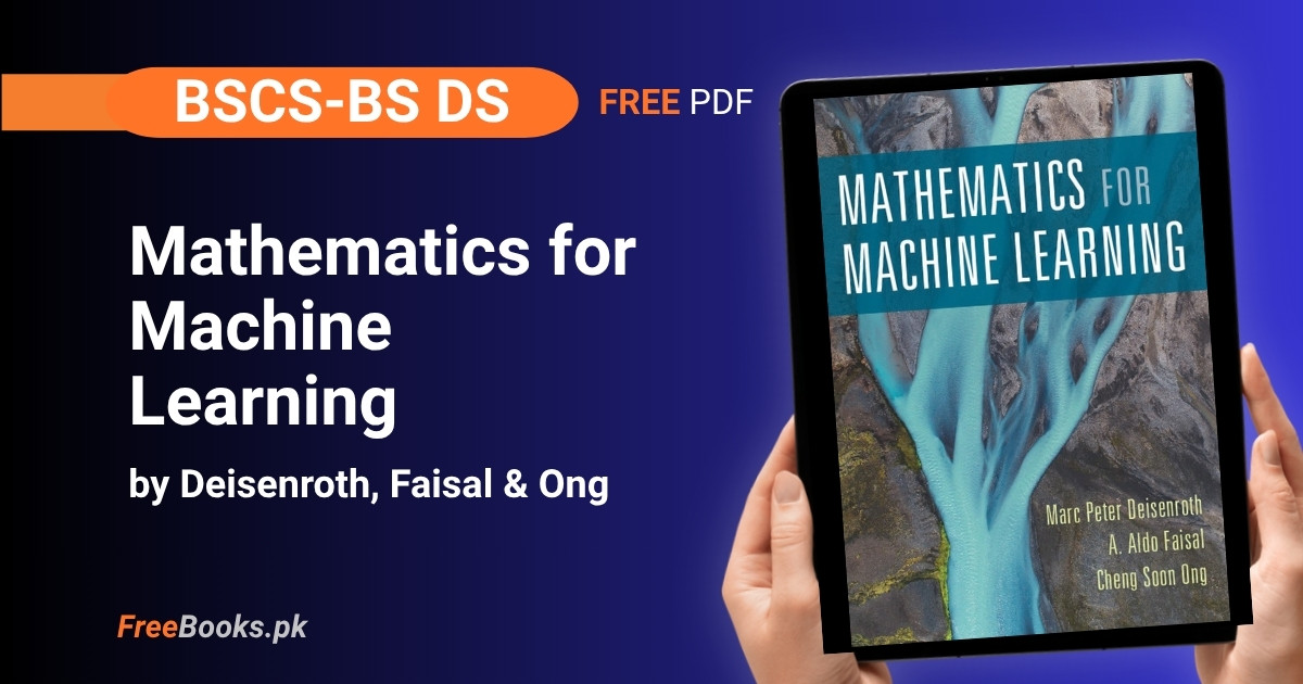
BS Computer Science and BS Data Science students can download Mathematics for Machine Learning by Marc Peter Deisenroth, A. Aldo Faisal and Cheng Soon Ong, published by Cambridge University Press and kept freely available online by the authors themselves. The book covers exactly the mathematics a machine learning course assumes going in — linear algebra, analytic geometry, matrix decompositions, vector calculus, probability and distributions, and continuous optimization — building each topic from precise definitions rather than skipping straight to code.
What sets this book apart for exam preparation is its two-part structure: Part I lays the mathematical foundations end-to-end, and Part II applies them directly to four core machine learning problems — regression, dimensionality reduction, density estimation, and classification — so a BSCS or BS Data Science student sees exactly why each theorem matters before meeting it again in a machine learning course. Pen-and-paper exercises close every Part I chapter, and Part II is paired with runnable Jupyter notebook tutorials instead, which suits both a pure math-for-ML course and a course that leads straight into a machine learning class.
Book Overview
| Course | Mathematics for Machine Learning |
| Degree Programs | BS Computer Science, BS Data Science |
| Level | University — the book’s own stated aim is to bridge the gap between high-school mathematics and the mathematics level a standard machine learning textbook assumes; no prior machine learning knowledge is required |
| Edition | Continuously updated free PDF, dated Draft (2024-01-15); based on the print edition published by Cambridge University Press in April 2020. A separate PDF matching the physical printed book is also offered by the authors. |
| Author(s) | Marc Peter Deisenroth, A. Aldo Faisal, Cheng Soon Ong |
| Structure | 12 chapters in two parts — Part I: Mathematical Foundations (Chapters 1–7), Part II: Central Machine Learning Problems (Chapters 8–12) |
| Exercises | Pen-and-paper exercises at the end of every Part I chapter (Chapters 2–7); Part II is paired with Jupyter notebook tutorials (Linear Regression, PCA, Gaussian Mixture Models) instead of end-of-chapter exercises |
| Language | English |
| License | Free to view and download for personal use only (Cambridge University Press) — not an open licence; no redistribution, resale, or derivative works permitted. © Deisenroth, Faisal & Ong, 2024. |
| Format | Free PDF (continuously updated, 417 pages), plus a separate PDF matching the printed edition; official source mml-book.com / mml-book.github.io |
Chapter List
Chapter 1: Introduction and Motivation
Difficulty: Easy · Key topics: predictors vs. training, data as vectors, models, bottom-up vs. top-down reading, the four pillars of machine learning
The book opens by warning that “machine learning algorithm” is genuinely ambiguous: it can mean a predictor that makes predictions from input data, or the training process that adapts that predictor’s internal parameters. From there it explains why data is treated as vectors throughout the book, describes a model as a simplified version of the real, unknown data-generating process, and compares training to climbing a hill toward a performance peak — while warning that performing well on training data is not the actual goal, since a model that has merely memorized its training set can fail badly on unseen data. The chapter closes by laying out the book’s own two-part structure: Part I builds the mathematical foundations, and Part II applies them to four “pillars” of machine learning.
Key Points:
- The phrase “machine learning algorithm” is used in two senses in this book: as a predictor (makes predictions) and as the training process that adapts a predictor’s parameters.
- The book treats data as vectors and a table of data as a matrix, so every later mathematical tool applies directly to real datasets.
- Training a model is compared to hill-climbing toward a performance-measure peak, but the real goal is performing well on unseen data, not memorizing the training set.
- Part I builds the foundations (linear algebra, analytic geometry, matrix decompositions, vector calculus, probability, optimization); Part II applies them to four pillars: regression, dimensionality reduction, density estimation, classification.
- The book can be read bottom-up (foundations first) or top-down (applications first, foundations as needed), since Part II chapters are only loosely coupled to each other.
Memory Tip: Keep the “predictor vs. training” split straight by asking which of the two a sentence is really about — a predictor makes a prediction; training changes the predictor’s parameters.
Common Mistake: Treating “machine learning algorithm” as one unambiguous term — the book explicitly warns this phrase means two different things depending on context, and conflating them causes real confusion in later chapters.
Important Questions:
- What are the two different things “machine learning algorithm” can mean in this book? A predictor that makes predictions from input data, and the training process that adapts the predictor’s parameters using data.
- What are the four pillars of machine learning covered in Part II? Regression, dimensionality reduction, density estimation, and classification.
Chapter 2: Linear Algebra
Difficulty: Medium · Key topics: vectors as abstract objects, systems of linear equations, matrices, vector spaces, linear independence, basis and rank, linear mappings, affine spaces
The chapter opens by generalizing “vector” beyond the school definition: geometric arrows, polynomials, and audio signals are all vectors because they can be added and scaled to produce another object of the same kind, alongside the more familiar elements of Rn. From there it works through solving systems of linear equations with matrix operations, defines vector spaces and subspaces formally, and studies which sets of vectors are linearly independent — leading to basis and rank, which pin down a vector space’s dimension. The chapter closes with linear mappings between vector spaces and affine spaces, both of which recur constantly for the rest of the book.
Key Points:
- A vector is any object that can be added to another of its kind and scaled by a real number to produce another object of the same kind — geometric arrows, polynomials, and audio signals all qualify.
- The book works mainly in
R^n, where vectors correspond directly to arrays of numbers, matching how data is stored on a computer. - A basis is a minimal linearly independent spanning set for a vector space, and the number of basis vectors (the rank) is the space’s dimension.
- A linear mapping preserves vector addition and scalar multiplication between two vector spaces, and can itself be represented as a matrix once bases are chosen.
- Affine spaces are vector spaces shifted away from the origin, which matters because many machine learning models are affine, not purely linear.
Memory Tip: Whenever you see “vector,” ask “vector of what” — once you check that addition and scalar multiplication produce another object of the same kind, you can treat polynomials, signals, or arrays with the exact same linear algebra toolbox.
Common Mistake: Assuming linear algebra only concerns arrays of numbers, then being confused when the book calls polynomials or functions “vectors” — the defining property is the two operations, not the shape of the object.
Important Questions:
- What two properties must an object satisfy to be called a vector in this book? It must be closed under addition (adding two of them gives another of the same kind) and closed under scalar multiplication.
- What is the relationship between a basis and the dimension of a vector space? The number of vectors in any basis of a vector space equals that space’s dimension; a basis is the smallest linearly independent set that spans the space.
Chapter 3: Analytic Geometry
Difficulty: Medium · Key topics: norms, inner products, lengths and distances, angles and orthogonality, orthonormal basis, orthogonal complement, orthogonal projections, rotations
The chapter formalizes the intuitive length of a geometric vector using a norm, defined by three properties — absolute homogeneity, the triangle inequality, and positive definiteness — and works through the Manhattan and Euclidean norms as concrete examples, adopting the Euclidean norm as the book’s default. Inner products are introduced next, which let the book define both length and the angle between two vectors, with orthogonality falling out as the special case where an inner product is zero. The chapter then builds orthonormal bases and orthogonal projections, closing with rotations — all of it feeding directly into the eigenvalue and PCA chapters that follow later in the book.
Key Points:
- A norm assigns every vector a nonnegative length and must satisfy three properties: absolute homogeneity, the triangle inequality, and positive definiteness.
- The Manhattan norm sums absolute coordinate values; the Euclidean norm is the default norm used throughout the book and equals the square root of a vector’s inner product with itself.
- An inner product defines both the length of a vector and the angle between two vectors, and two vectors are orthogonal exactly when their inner product is zero.
- An orthogonal projection maps a vector onto a subspace so that the projection error is itself orthogonal to that subspace — the geometric idea Chapter 10 builds Principal Component Analysis on.
- Orthonormal bases (orthogonal, unit-length vectors) simplify almost every computation later in the book, from coordinate representation to rotations.
Memory Tip: “Orthogonal means the leftover is perpendicular” — an orthogonal projection is correct exactly when the error vector (original minus projection) is orthogonal to the subspace you projected onto; that single check verifies any projection computation.
Common Mistake: Confusing a norm with an inner product — every inner product induces a norm, but not every norm comes from an inner product (the Manhattan norm does not), so norm properties alone cannot be used to compute an angle.
Important Questions:
- What three properties must a function satisfy to be called a norm? Absolute homogeneity, the triangle inequality, and positive definiteness.
- When are two vectors called orthogonal? When their inner product equals zero.
Chapter 4: Matrix Decompositions
Difficulty: Hard · Key topics: determinant and trace, eigenvalues and eigenvectors, Cholesky decomposition, eigendecomposition and diagonalization, singular value decomposition (SVD), matrix approximation
The chapter opens with the determinant as a direct invertibility test, worked through explicitly for a 2×2 matrix (invertible exactly when a11a22 − a12a21 ≠ 0), before moving to eigenvalues and eigenvectors and the conditions under which a matrix can be diagonalized. Cholesky decomposition, the tool that makes sampling from Gaussian distributions in Chapter 6 practical, follows, and the chapter’s own mind map explicitly traces a path from determinant to eigenvalues to diagonalization to Singular Value Decomposition (SVD), which Chapter 10 later uses to derive PCA. The chapter closes with low-rank matrix approximation, the same idea that lets PCA compress high-dimensional data.
Key Points:
- The determinant of a square matrix tests invertibility directly: a matrix is invertible if and only if its determinant is nonzero.
- Eigenvalues and eigenvectors satisfy
Av = λv, and a matrix is diagonalizable exactly when it has enough linearly independent eigenvectors to form a basis. - Cholesky decomposition factors a symmetric, positive-definite matrix into a lower-triangular matrix times its own transpose, which is what makes sampling from a Gaussian distribution in Chapter 6 computationally practical.
- Singular Value Decomposition (SVD) factors any matrix — not just square ones — and is the tool Chapter 10 uses to compute Principal Component Analysis.
- Low-rank matrix approximation keeps only the largest singular values of a matrix’s SVD, the same idea PCA uses to compress high-dimensional data.
Memory Tip: Follow the chapter’s own mind map — determinant tells you invertibility, invertibility feeds eigenvalues, eigenvalues feed diagonalization, and diagonalization is the special case of SVD that PCA in Chapter 10 actually needs.
Common Mistake: Assuming every matrix can be diagonalized — only matrices with a full set of linearly independent eigenvectors can be; SVD exists for every matrix, which is exactly why it is the more generally useful decomposition.
Important Questions:
- How do you test whether a 2×2 matrix is invertible? Compute its determinant, a11a22 − a12a21; the matrix is invertible exactly when this value is nonzero.
- What is the key difference between eigendecomposition and singular value decomposition? Eigendecomposition requires a square matrix with enough independent eigenvectors and diagonalizes it using its own eigenvectors; SVD works for any matrix at all, using two different sets of singular vectors.
Chapter 5: Vector Calculus
Difficulty: Hard · Key topics: difference quotient, partial derivatives and gradients, gradients of vector-valued functions and matrices, chain rule identities, backpropagation and automatic differentiation, Taylor series
The chapter starts from first principles: the derivative of a univariate function is defined as the limit of the difference quotient as the step size shrinks to zero, the incline of a secant line collapsing onto the tangent. It then generalizes to the gradient, which collects every partial derivative of a multivariate function into one vector pointing in the direction of steepest ascent, and extends this to vector-valued functions (producing a Jacobian) and even to functions of matrices. Backpropagation is presented explicitly as an application of the chain rule, computed efficiently by automatic differentiation, and the chapter closes with multivariate Taylor series, which linearize a function locally around a point — exactly what gradient descent in Chapter 7 relies on.
Key Points:
- The derivative of a univariate function is the limit of the difference quotient δy/δx as δx approaches zero — the secant line’s incline shrinking to the tangent line’s.
- The gradient collects all partial derivatives of a multivariate function into a single vector, and it points in the direction of steepest ascent of that function.
- Gradients extend to vector-valued functions (producing a Jacobian matrix) and even to functions of matrices, both of which machine learning models need directly.
- Backpropagation is presented as an application of the chain rule, computed efficiently by automatic differentiation rather than by hand-deriving each gradient.
- A multivariate Taylor series linearizes a function around a point using its gradient (and higher-order derivatives), which is exactly what gradient-descent optimization in Chapter 7 relies on locally.
Memory Tip: “Gradient = uphill direction” — whenever a later chapter asks you to minimize something, remember the gradient itself points toward increasing the function, so optimization moves against it.
Common Mistake: Computing a gradient and forgetting it is a direction of steepest ascent, not descent — students then add the gradient instead of subtracting it when writing a gradient-descent update rule in Chapter 7.
Important Questions:
- What does the difference quotient become as δx approaches zero? The derivative of the function at that point — the slope of the tangent line rather than the secant line.
- Why is automatic differentiation used for backpropagation instead of deriving each gradient by hand? Because it applies the chain rule mechanically and efficiently across a whole computation graph, avoiding the error-prone, unscalable work of deriving every partial derivative by hand.
Chapter 6: Probability and Distributions
Difficulty: Hard · Key topics: probability space construction, discrete and continuous probabilities, sum rule/product rule/Bayes’ theorem, summary statistics and independence, Gaussian distribution, conjugacy and exponential family, change of variables
The chapter frames probability as a generalization of Boolean logic to degrees of plausibility, illustrated with its own example of a friend running late: logically ruling out “on time,” then judging “delayed by traffic” far more plausible than “abducted by aliens” without any strict logical requirement to do so. From there it builds the sum rule, product rule, and Bayes’ theorem, then covers summary statistics, independence, and dedicates an entire section to the Gaussian distribution because so many later chapters need its closed-form results. The chapter closes with conjugate distributions and the exponential family, which keep Bayesian updating tractable by hand, and change of variables for transforming distributions.
Key Points:
- Probability theory is presented as a generalization of Boolean logic to degrees of plausibility, following E. T. Jaynes’s criteria for representing plausible reasoning consistently with real numbers.
- The sum rule, product rule, and Bayes’ theorem are the three rules the whole chapter is built on; Bayes’ theorem is what lets new evidence update a prior belief into a posterior belief.
- Independence and summary statistics (mean, variance, covariance) describe a distribution compactly without needing its full functional form.
- The Gaussian distribution gets its own dedicated section because closed-form results (needed for linear regression in Chapter 9 and Gaussian mixture models in Chapter 11) are far easier to derive for it than for most other distributions.
- Conjugate distributions and the exponential family are introduced because a conjugate prior keeps the posterior in the same distribution family after seeing data, which is what makes Bayesian updating tractable by hand.
Memory Tip: Picture the friend running late — ruling out “on time” is deductive logic, but judging “delayed by traffic” more likely than “abducted by aliens” is exactly the plausible reasoning Bayes’ theorem formalizes with numbers instead of intuition.
Common Mistake: Confusing the product rule (which always holds) with independence (a special case where it simplifies), then wrongly multiplying two probabilities together for events that are not actually independent.
Important Questions:
- What are the three rules of probability the chapter is organized around? The sum rule, the product rule, and Bayes’ theorem.
- Why does the book give the Gaussian distribution its own dedicated section? Because many operations on Gaussians (conditioning, marginalizing, combining) have closed-form solutions, which is essential for the linear regression and Gaussian mixture model chapters later in the book.
Chapter 7: Continuous Optimization
Difficulty: Hard · Key topics: gradient descent, step size, momentum, stochastic gradient descent, Lagrange multipliers, constrained optimization, convex optimization and duality
The chapter’s own worked example — a cubic objective function with three stationary points — shows gradient descent’s central weakness directly: starting on the wrong side of a local maximum leads the algorithm to converge on the wrong, worse local minimum, and the second derivative test is used to tell a minimum from a maximum at each stationary point. Step size is introduced as a decision separate from direction, and convex functions are singled out specifically because they remove the starting-point dependency — every local minimum of a convex function is the global minimum. The chapter closes with constrained optimization via Lagrange multipliers, the exact tool Chapter 10 later uses to derive PCA.
Key Points:
- Gradient descent follows the negative gradient of an objective function, but the chapter’s own worked example shows starting on the wrong side of a local maximum leads gradient descent to the wrong local minimum.
- The second derivative test distinguishes a minimum from a maximum at a stationary point: positive means minimum, negative means maximum.
- Step size (how far to move along the negative gradient) is a separate decision from direction, and choosing it badly is a common source of slow or unstable convergence.
- Convex functions are introduced specifically because they remove the starting-point dependency problem — for a convex function, every local minimum is the global minimum.
- Constrained optimization uses Lagrange multipliers to fold constraints directly into the objective function being optimized, the exact tool Chapter 10 uses to derive PCA.
Memory Tip: “Convex means no wrong valleys” — on a convex objective, gradient descent can start anywhere and still reach the one true minimum, which is precisely why the chapter singles convexity out as special.
Common Mistake: Running gradient descent on a non-convex function and assuming the minimum it converges to is the global minimum — the chapter’s own cubic example shows a starting point can lead gradient descent straight to a worse local minimum.
Important Questions:
- How does the second derivative at a stationary point tell you whether it is a minimum or a maximum? A positive second derivative means the stationary point is a minimum; a negative second derivative means it is a maximum.
- Why do convex functions matter for gradient descent? Because for a convex function every local minimum is also the global minimum, removing the dependency on where the optimization starts that a non-convex function creates.
Chapter 8: When Models Meet Data
Difficulty: Medium · Key topics: data as vectors, tabular data, empirical risk minimization, parameter estimation, probabilistic modeling and inference, directed graphical models, model selection
Part II opens with the chapter’s own example of a messy human-resources table — name, gender, degree, postcode, age, salary — to make the point that real data is rarely already numeric: categorical columns like gender must be explicitly encoded (0/1 or −1/+1) before any of Part I’s linear algebra tools apply. The chapter restates data, models, and learning from Chapter 1 in mathematical terms, then previews empirical risk minimization, maximum likelihood estimation, probabilistic modeling, and directed graphical models as a visual language for expressing which variables in a model depend on which others. It closes with model selection, framed explicitly as a guard against overfitting.
Key Points:
- Real data (the chapter’s own human-resources example: name, gender, degree, postcode, age, salary) is rarely already numeric — categorical columns like gender must be encoded as numbers before any linear algebra tool applies.
- Empirical risk minimization picks model parameters that minimize an average loss over the observed training data.
- Maximum likelihood estimation and probabilistic modeling frame the same fitting problem in terms of probability distributions rather than a loss function directly.
- Directed graphical models give a visual language for writing down which variables in a probabilistic model depend on which others, without writing out the full joint distribution by hand.
- Model selection compares different models (and parametrizations of the same model) to find the simplest one that still explains the training data well, guarding against overfitting.
Memory Tip: Before touching any formula from Part I, ask “is this column actually a number yet” — the chapter’s own salary/gender/postcode table is the reminder that real data needs encoding decisions before it becomes the vectors the rest of the book assumes.
Common Mistake: Treating “more flexible model” as automatically “better model” — the chapter’s model selection section exists specifically because an overly flexible model fits training data closely while performing worse on unseen data.
Important Questions:
- Why can’t the human-resources example table be fed directly into a machine learning model? Because columns like gender are categorical, not numerical, and must first be converted into a numerical representation before vector and matrix operations apply.
- What is empirical risk minimization? Choosing model parameters that minimize the average loss of the model’s predictions over the observed training dataset.
Chapter 9: Linear Regression
Difficulty: Medium · Key topics: problem formulation, maximum likelihood parameter estimation, Bayesian linear regression, maximum likelihood as orthogonal projection
The chapter opens by listing where regression actually shows up — time-series analysis, robotics and control, optimization, deep-learning applications — before writing a single equation, to make the point that the same mathematical problem recurs everywhere. It separates choosing a model class from finding good parameters for that class, connects overfitting directly back to the model selection idea from Chapter 8, and contrasts maximum likelihood estimation (one best-fit answer) with Bayesian linear regression, which integrates the parameters out instead of optimizing them, producing genuine prediction uncertainty. The chapter closes by showing that maximum likelihood estimation for linear regression is itself equivalent to an orthogonal projection, tying the whole chapter back to Chapter 3.
Key Points:
- Regression is framed broadly — the chapter lists time-series analysis, robotics and control, optimization, and deep-learning applications before ever writing an equation.
- Choosing the regression model class (e.g. which polynomial degree) is treated as a separate decision from finding good parameters for that chosen class.
- Overfitting happens when a regression function fits the training data too well but fails to generalize, connecting directly back to the model selection idea from Chapter 8.
- Bayesian linear regression integrates out the parameters instead of optimizing a single best value for them, producing a measure of prediction uncertainty that plain maximum likelihood estimation does not.
- Maximum likelihood estimation for linear regression is shown to be equivalent to an orthogonal projection, tying the chapter back to the projections introduced in Chapter 3.
Memory Tip: “Bayesian regression keeps the uncertainty, maximum likelihood throws it away” — maximum likelihood picks one best-fit line; Bayesian linear regression keeps a whole distribution over plausible lines, which is what lets it report how confident a prediction actually is.
Common Mistake: Reporting a maximum likelihood regression prediction without any uncertainty, then being surprised the model is confidently wrong on a test point far from the training data — Bayesian linear regression exists precisely to address this gap.
Important Questions:
- What does it mean for maximum likelihood estimation in linear regression to be equivalent to an orthogonal projection? The best-fit prediction is geometrically the projection of the observed outputs onto the subspace spanned by the model’s basis functions, directly using the orthogonal projection idea from Chapter 3.
- Why does Bayesian linear regression integrate out the parameters instead of optimizing them? To keep a full distribution over plausible parameter values rather than a single point estimate, giving a genuine measure of confidence in the model’s predictions.
Chapter 10: Dimensionality Reduction with Principal Component Analysis
Difficulty: Hard · Key topics: problem setting, maximum variance perspective, projection perspective, eigenvector computation and low-rank approximation, PCA in high dimensions, latent variable perspective
PCA is motivated by the chapter’s own example: high-dimensional data such as images often varies little along most directions, so it can be represented almost losslessly in far fewer dimensions. The chapter sets up the problem as finding an orthonormal projection matrix whose columns span a lower-dimensional subspace, then derives PCA from two equivalent angles — maximizing the variance of the projected data, and minimizing the reconstruction error — proving both give the same answer. It explicitly draws on five earlier chapters (basis and basis change, projections, eigenvalues, Gaussians, and constrained optimization) to derive PCA from first principles, and closes by noting PCA is also known as the Karhunen-Loève transform in signal processing.
Key Points:
- PCA is motivated by the observation that high-dimensional data (the chapter’s example: images) often varies little along most directions, so it can be represented almost losslessly in far fewer dimensions.
- The method finds an orthonormal projection matrix whose columns span a lower-dimensional subspace, minimizing the loss between the original data points and their projections.
- PCA can be derived from two equivalent angles: maximizing the variance of the projected data, or minimizing the reconstruction (projection) error — the chapter proves both give the same answer.
- The data covariance matrix’s eigenvectors are the directions PCA keeps, and its largest eigenvalues correspond to the directions of greatest variance in the data.
- PCA is also known as the Karhunen-Loève transform in signal processing, and the chapter explicitly draws on five earlier chapters (basis and basis change, projections, eigenvalues, Gaussians, constrained optimization) to derive it from first principles.
Memory Tip: “Keep the directions, drop the noise” — PCA keeps the eigenvector directions with the largest eigenvalues of the data covariance matrix, because those are the directions the data actually varies along.
Common Mistake: Forgetting to center the data (subtract the mean) before computing PCA — the whole derivation assumes a dataset with mean zero, and skipping this step silently produces a wrong covariance matrix and wrong principal directions.
Important Questions:
- What two equivalent ways does the chapter use to derive PCA? Maximizing the variance of the projected data (maximum variance perspective) and minimizing the reconstruction error between original and projected points (projection perspective).
- What do the eigenvectors of the data covariance matrix represent in PCA? The directions of the lower-dimensional subspace the data is projected onto, ordered by how much variance in the data each direction captures.
Chapter 11: Density Estimation with Gaussian Mixture Models
Difficulty: Hard · Key topics: Gaussian mixture model, maximum likelihood parameter learning, EM algorithm, latent-variable perspective
The chapter opens by noting a single Gaussian distribution is a poor fit for data with multiple clusters, motivating a more expressive family: mixture models, defined as a convex combination of K simple base distributions with weights that sum to one. Focusing on Gaussian mixture models, the chapter shows that setting K = 1 recovers an ordinary Gaussian as a special case, connecting directly back to Chapter 6, but that unlike linear regression or PCA, maximizing a GMM’s likelihood has no closed-form solution — it produces a set of dependent simultaneous equations that can only be solved iteratively. This is why the chapter builds toward the EM (Expectation-Maximization) algorithm as its central tool.
Key Points:
- A single Gaussian distribution is a poor fit for data with multiple clusters, which is exactly why the chapter introduces mixture models as a more expressive family.
- A Gaussian Mixture Model is a convex combination of K Gaussian components, each with its own mean and covariance, weighted by mixture weights that sum to one.
- Setting K = 1 in the mixture model recovers a single ordinary Gaussian distribution as a special case, connecting directly back to Chapter 6.
- Unlike linear regression or PCA, maximizing the likelihood of a GMM’s parameters has no closed-form solution — it leads to a set of dependent simultaneous equations that must be solved iteratively.
- The EM (Expectation-Maximization) algorithm is the iterative scheme the chapter uses to solve this, alternating between assigning soft cluster responsibilities and updating each component’s parameters.
Memory Tip: “One Gaussian, one hump — mixtures give you many” — whenever a dataset visibly has multiple clusters, that is the signal a single Gaussian (Chapter 6) cannot capture it, and a Gaussian mixture model is what to reach for.
Common Mistake: Expecting to solve a GMM’s maximum likelihood parameters directly by setting a gradient to zero, the way linear regression is solved in Chapter 9 — the chapter is explicit that no closed-form solution exists, which is precisely why the EM algorithm is needed.
Important Questions:
- What happens to a Gaussian Mixture Model when K = 1? It reduces to a single ordinary Gaussian distribution, showing a GMM strictly generalizes the Gaussian case from Chapter 6.
- Why does fitting a Gaussian Mixture Model require an iterative algorithm instead of a closed-form solution? Because maximizing its likelihood produces a set of simultaneous equations whose parameters depend on each other, which the EM algorithm solves by iterating rather than by direct computation.
Chapter 12: Classification with Support Vector Machines
Difficulty: Hard · Key topics: separating hyperplanes, primal SVM, dual SVM, kernels, numerical solution
The chapter opens with a deliberate contrast to Chapter 9: instead of the probabilistic, maximum-likelihood view of regression, Support Vector Machines approach classification geometrically, designing a loss function directly from geometric intuition about separating hyperplanes. A hyperplane — an affine subspace one dimension smaller than the space it lives in — separates two classes of labeled examples, and because the SVM optimization problem has no analytic solution, the chapter relies directly on the optimization tools from Chapter 7. It then develops the dual SVM formulation, which reframes training in terms of inner products between training examples, opening the door to kernels that let an SVM classify data that is not linearly separable in its original space.
Key Points:
- Support Vector Machines approach classification geometrically rather than probabilistically — a deliberate contrast with the maximum likelihood view of regression in Chapter 9.
- A hyperplane is an affine subspace of one dimension less than the space it lives in, and it is what an SVM uses to separate two classes of labeled examples.
- Because the SVM optimization problem has no analytic solution, the chapter relies directly on the optimization tools introduced in Chapter 7.
- The dual SVM formulation reframes training in terms of inner products between training examples, which is what makes the kernel trick possible.
- Kernels let an SVM classify data that is not linearly separable in its original space, by implicitly working in a higher-dimensional space without ever computing the transformed vectors directly.
Memory Tip: “Primal fits parameters, dual fits examples” — the primal SVM optimizes directly over the hyperplane’s parameters, while the dual formulation rewrites the same problem in terms of inner products between training examples, the version kernels attach to.
Common Mistake: Assuming a hyperplane in SVM classification always means a simple 2D line the way an introductory figure draws it — a hyperplane is one dimension less than the full feature space, so in a real dataset with many features it is a much higher-dimensional cut, not a line.
Important Questions:
- How does the SVM’s approach to classification differ from the linear regression approach in Chapter 9? SVM reasons geometrically, designing a loss function directly from geometric intuition about separating hyperplanes, rather than starting from a probabilistic model of the data as maximum likelihood does.
- Why does the dual SVM formulation matter for using kernels? Because the dual formulation expresses training only in terms of inner products between examples, and kernels replace that inner product with a function that implicitly computes it in a higher-dimensional space, without ever forming the transformed vectors.
Download Mathematics for Machine Learning PDF (Free)
This book is free to view and download from its official source. Click below to open the continuously updated PDF directly from the authors’ own site — the version they describe as the most up to date, ahead of typo fixes in the printed edition.
↓ Download PDFHow to Study This Book
The book itself offers two ways to read it, and both work: bottom-up, working straight through Part I before touching Part II, or top-down, picking a Part II chapter you care about and reading backward into the Part I chapters it needs. Part I chapters mostly build on each other in order, but Part II chapters are only loosely coupled, so it is genuinely fine to jump to whichever of Chapters 9–12 matches your course syllabus first.
Chapters 2 and 3 (Linear Algebra, Analytic Geometry) are the computational core almost everything else depends on. Read them in order and do every exercise — vector spaces, bases, norms, inner products and orthogonal projections are used without re-explanation in every chapter that follows, including both matrix decompositions in Chapter 4 and PCA in Chapter 10.
Chapter 4 (Matrix Decompositions) is worth reading slowly even on a first pass, because its own mind map is effectively a map of the rest of the book: determinant → eigenvalues → diagonalization → SVD is the exact chain Chapter 10 needs for PCA, and Cholesky decomposition is what makes the Gaussian sampling in Chapter 6 practical.
Chapters 5 and 7 (Vector Calculus, Continuous Optimization) should be read as a pair even though one chapter separates them — Chapter 5 builds the gradient, and Chapter 7 is where that gradient is put to work in gradient descent and Lagrange multipliers. If your calculus is rusty, it is worth reviewing differentiation before Chapter 5 rather than during it.
Chapter 6 (Probability and Distributions) is the longest and most demanding chapter in Part I. Its Gaussian distribution section (6.5) deserves particular attention, since Chapters 9 and 11 both lean on Gaussian results derived there without re-deriving them.
In Part II, match the chapter to what your machine learning course needs: Chapter 9 (Linear Regression) needs Chapters 3, 6 and 7; Chapter 10 (PCA) needs Chapters 2, 3, 4, 6 and 7 together, which the chapter states explicitly; Chapter 11 (Gaussian Mixture Models) needs Chapters 5, 6 and 7; and Chapter 12 (SVMs) needs Chapters 3 and 7. None of the four Part II chapters requires all of Part I at once.
Do the pen-and-paper exercises at the end of every Part I chapter (Chapters 2–7) before moving on — they are how the book checks whether a definition has actually been understood, not just read. For Part II, run the official Jupyter notebook tutorials (Linear Regression, PCA, Gaussian Mixture Models, all linked from the official site) instead of looking for end-of-chapter exercises, since the book pairs code, not problem sets, with these four chapters.
Know what this book does not do: by the authors’ own stated aim, it covers only four machine learning problems in depth and is explicitly meant as a bridge into other, fuller machine learning textbooks — not a substitute for one. A student who needs neural network architectures, modern deep learning methods, or a broader survey of ML algorithms should treat this book as preparation and pair it with a dedicated machine learning or deep learning textbook afterward.
Used In These Programs
This book is used for the Mathematics for Machine Learning course in: BS Computer Science. Browse all Machine Learning books or all Mathematics books.
Who Should Read This
This book suits a BS Computer Science or BS Data Science student who is about to take — or is already struggling in — a machine learning course and needs the mathematics under it explained properly rather than assumed. It assumes only high-school mathematics going in, but moves quickly to a proof-and-definition style that a student whose calculus is rusty should not underestimate; reviewing Calculus Volume 1 before Chapter 5 (Vector Calculus) is worth the time if differentiation itself feels shaky. It is not a machine learning textbook in the usual sense: the authors deliberately cover only four ML problems in depth (regression, dimensionality reduction, density estimation, classification) rather than surveying algorithms broadly, so a student wanting a full ML methods course should treat this as the mathematical preparation for that course, not a replacement for it. Students already comfortable with undergraduate linear algebra and probability can skip straight to Part II and use Part I chapters as a reference when a specific tool is unfamiliar.
Applicable Universities
This book is useful for students at Pakistani universities offering BS Computer Science and BS Data Science including Punjab University, Virtual University, COMSATS, FAST, UET, NUST, and other HEC-recognized institutions.
FAQs
Is Mathematics for Machine Learning free?
Yes, to view and download for personal use. The book’s own copyright page states this exactly: “This version is free to view and download for personal use only. Not for re-distribution, re-sale, or use in derivative works.” That is not a Creative Commons or open licence — Cambridge University Press and the authors keep full copyright — but the PDF itself costs nothing and needs no account or payment to download.
Which edition is this?
The free PDF is a continuously updated “Draft,” dated 2024-01-15 on its own copyright page, kept current past the original April 2020 Cambridge University Press print edition. The authors separately host a second PDF that matches the physical printed book exactly (useful if your course cites page numbers from the print edition), while the main PDF keeps fixing typos and errata beyond it.
How many chapters does it have, and does it have exercises?
12 chapters across two parts: Part I (Chapters 1–7) covers the mathematical foundations, and Part II (Chapters 8–12) applies them to four machine learning problems. Pen-and-paper exercises are provided at the end of every Part I chapter; Part II is paired with Jupyter notebook programming tutorials instead of a written exercise set.
Is it good for complete beginners?
It assumes only high-school mathematics to start, by the authors’ own design — but it moves quickly into a precise, proof-and-definition academic style rather than a gentle walkthrough. A student who has never seen a mathematical proof, or whose calculus is rusty, should expect to slow down significantly in Chapters 4 through 7, not just skim them.
Does it cover linear algebra and probability in depth?
Yes, both get full chapters (Chapter 2: Linear Algebra, Chapter 6: Probability and Distributions) built from first principles, not a quick refresher. Chapter 6 in particular is the longest chapter in the book, since Chapters 9 and 11 both depend on its Gaussian distribution results.
Does this book teach machine learning algorithms, or just the math?
Mostly the math. The authors state explicitly that they cover only four representative machine learning problems in depth — linear regression, PCA, Gaussian mixture models, and SVM classification — specifically so a reader can go on to read a full machine learning textbook with the mathematics no longer in the way. It is meant as preparation for an ML course or textbook, not a replacement for one.
Related Books
- Calculus Volume 1 – Strang & Herman (OpenStax)
- Calculus Volume 2 – Strang & Herman (OpenStax)
- Discrete Mathematics: An Open Introduction – Oscar Levin (4th Edition)
Mathematics for Machine Learning is the rare free textbook that names its job precisely: not to teach machine learning algorithms, but to make sure the mathematics under them — linear algebra, calculus, probability, and optimization — is actually understood before a student opens a standard ML textbook. Its two-part structure, four worked ML problems, and honest scope make it a strong bridge course for BSCS and BS Data Science students. Browse more Mathematics books for the rest of your semester.
Mathematics for Machine Learning, by Marc Peter Deisenroth, A. Aldo Faisal and Cheng Soon Ong. Published by Cambridge University Press (2020). Free to view and download for personal use only, not for redistribution, resale, or use in derivative works. © Deisenroth, Faisal & Ong, 2024. Official source: https://mml-book.com / https://mml-book.github.io/
© Copyright Policy
Freebooks.pk is an educational resource for students in Pakistan. Textbooks and other books belong to their respective boards, authors and publishers, and all rights remain with them. If you are the copyright holder of any material on this page and want it changed or removed, please contact us or file a request under our DMCA policy. We review every request and remove reported content promptly.