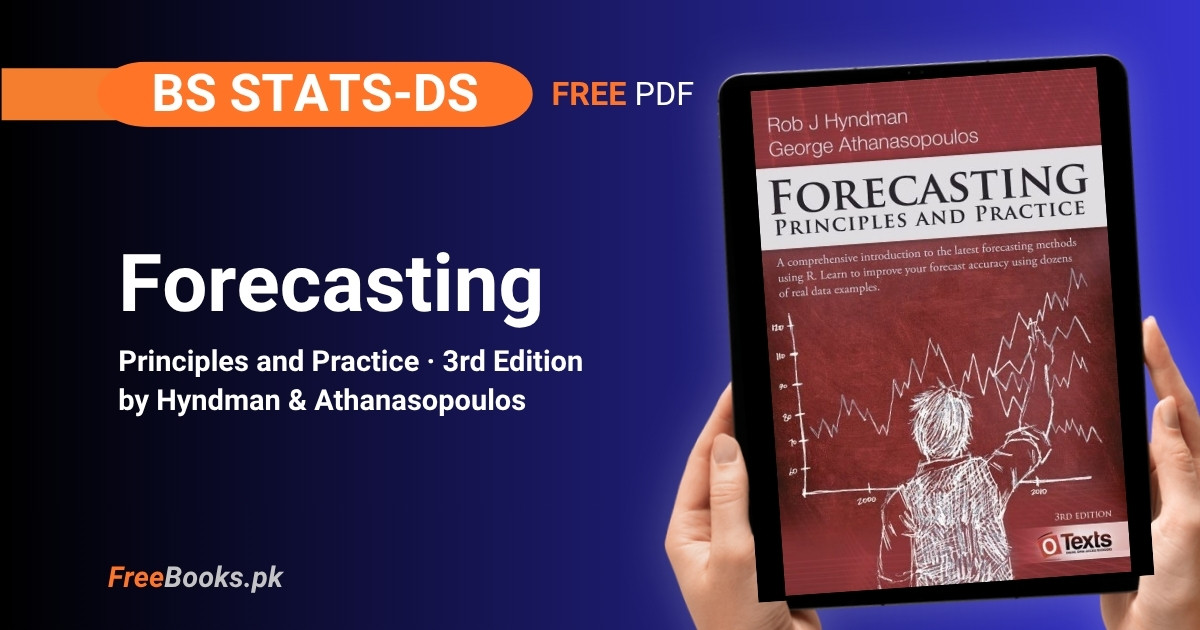
Students in a BS Statistics, BS Data Science, or BS Computer Science program taking a Time Series Analysis or Business Forecasting course can read the complete 3rd edition of “Forecasting: Principles and Practice” (widely known by its short name, FPP3), by Rob J Hyndman and George Athanasopoulos of Monash University, Australia, free at its official source, otexts.com/fpp3. It is a 13-chapter book that takes a reader from time series graphics and decomposition through the two workhorse forecasting model families, exponential smoothing (ETS) and ARIMA, and on to regression-based, hierarchical, and several advanced forecasting methods, using the R programming language throughout via the tidyverse-integrated tsibble, feasts and fable packages.
FPP3 is one of the most widely used open forecasting textbooks in the world, assigned in university courses well beyond Monash, and is the book behind the popular fable and tsibble R packages themselves. It is free and continuously updated online — corrections and new material appear without waiting for a numbered new edition — but it does not offer a downloadable PDF; the free version is HTML-only, with a separate paid print edition sold through Amazon for readers who want a physical copy. The book’s own pages carry no explicit open-source licence statement, so this page credits the authors and OTexts directly rather than naming a specific Creative Commons licence.
Book Overview
| Course | Time Series Analysis / Business & Statistical Forecasting |
| Degree Programs | BS Statistics, BS Data Science; also used as an advanced forecasting elective within BS Computer Science and BS Data Science programs |
| Level | University — intermediate to advanced; assumes introductory statistics and high-school algebra, with a few sections flagged as needing basic matrix algebra |
| Edition | 3rd edition — online edition continuously updated (last revised 16 September 2026); print edition last updated 31 May 2021 |
| Author(s) | Rob J Hyndman & George Athanasopoulos (Monash University, Australia) |
| Structure | 13 numbered chapters, Getting Started through Some Practical Forecasting Issues, plus an appendix on using R — no separately labeled parts |
| Exercises | End-of-chapter exercises and a Further Reading list in every chapter; full instructor solutions available to verified university instructors only |
| Language | English |
| Format | Free, continuously-updated official HTML edition only — no free PDF is offered; a paid print edition is sold separately via Amazon |
Chapter List
Chapter 1: Getting Started
Difficulty: Easy · Key topics: predictability, forecasting vs. planning, five-step forecasting task, random variable, point forecast, prediction interval
Chapter 1 opens with forecasting’s long, strange history — from the Oracle at Delphi to a Roman emperor’s AD 357 ban on consulting soothsayers — and famous failed predictions about computing, including a 1977 claim from DEC’s president that no one would want a computer at home. It argues predictability depends on four factors: how well the underlying process is understood, how much data exists, how similar the future is likely to be to the past, and whether the act of forecasting changes the outcome itself. It lays out the five basic steps of any forecasting task, from problem definition through choosing and fitting a model, and introduces the book’s core statistical idea: a future value is treated as a random variable, so a forecast is the middle of a range of possible futures, reported with a prediction interval rather than one bare number.
Key Points:
- Predictability depends on four things: understanding of the process, amount of data, how similar the future is to the past, and whether the forecast itself affects the outcome.
- A forecasting task has five basic steps: problem definition, gathering information, exploratory analysis, choosing and fitting models, and using and evaluating a forecasting model.
- The book treats the value being forecast,
y_t, as a random variable, writteny_t | Igiven everything known asI. - A point forecast is the middle of the range of possible future values; a prediction interval (e.g. 95%) gives a range expected to contain the true value with that probability.
- Uncertainty about a forecast generally grows the further ahead it is made.
Practice Tip: Before opening R, write out the five basic steps for a forecasting problem you already understand — such as next month’s household electricity bill — naming the data, the model choice, and how you would evaluate it. Every later chapter’s R workflow follows this same shape.
Common Mistake: Reporting only a single point forecast and treating it as a guaranteed outcome — a defensible forecast is a distribution of plausible futures with a stated prediction interval, not one number pretending to be certain.
Important Questions:
- What four factors determine how predictable something is, according to Chapter 1? How well the contributing factors are understood, how much data is available, how similar the future is expected to be to the past, and whether the forecast itself can influence the outcome being forecast.
- What are the five basic steps of a forecasting task? Problem definition, gathering information, preliminary (exploratory) analysis, choosing and fitting models, and using and evaluating a forecasting model.
Chapter 2: Time Series Graphics
Difficulty: Easy · Key topics: tsibble, time plots, trend, seasonal, cyclic, seasonal subseries plots, lag plots, autocorrelation (ACF), white noise
Chapter 2 sets up the book’s data structure, the tsibble, which pairs observations with an explicit time index and works throughout the tidyverse. It then works through the graphs used to explore a series before any model is fitted: time plots, seasonal plots and seasonal subseries plots for spotting recurring patterns, scatterplots and lag plots for relationships between a series and its own past, and the autocorrelation function (ACF) for measuring how strongly a series relates to its own lagged values. The chapter carefully distinguishes trend, seasonal and cyclic behaviour, since a cyclic pattern (no fixed period, usually tied to the business cycle) is often confused with a seasonal one (a fixed, calendar-based period). It closes by defining white noise, a series with no autocorrelation, which every later model’s residuals should resemble.
Key Points:
- A
tsibbleobject pairs data with an explicit timeindex, extending a tidy tibble with temporal structure. - Trend is any long-term increase or decrease; seasonal is a fixed, calendar-linked pattern; cyclic is a rise-and-fall with no fixed period, usually tied to the business cycle and generally lasting two years or more.
- The
ACF()function computes autocorrelation coefficientsr_1, r_2, ...measuring the correlation betweeny_tandy_(t-k)at each lagk. - For a white noise series, about 95% of ACF spikes should fall within ±1.96/√T of zero, where T is the series length.
- Seasonal subseries plots and lag plots reveal patterns a single time plot can hide, especially when several seasonal periods overlap.
Practice Tip: Run y |> ACF(x) |> autoplot() on any dataset before fitting a model to it — a spike at lag 4 on quarterly data or lag 12 on monthly data is the ACF confirming seasonality you may have only suspected from the time plot.
Common Mistake: Confusing a cyclic pattern with a seasonal one because both involve rises and falls — seasonality has a fixed, known period tied to the calendar, while a cycle’s length varies and is usually driven by economic conditions.
Important Questions:
- What is the key difference between seasonal and cyclic behaviour in a time series? Seasonality is always of a fixed and known period tied to the calendar (e.g. a yearly or weekly pattern); a cycle has no fixed frequency, and its rises and falls, usually linked to the business cycle, typically last two years or more.
- What does the ACF measure, and what does it look like for a white noise series? The ACF measures the correlation between a series and its own lagged values,
y_tandy_(t-k), at each lagk. For white noise, essentially no autocorrelation exists, so about 95% of the ACF’s spikes should lie within ±1.96/√T of zero.
Chapter 3: Time Series Decomposition
Difficulty: Medium · Key topics: Box-Cox transformation, trend-cycle, seasonal component, remainder, additive vs. multiplicative decomposition, moving averages, X-11/SEATS, STL
Chapter 3 splits a time series into a trend-cycle component, a seasonal component and a remainder, using either an additive model (y = S + T + R) when seasonal swings stay roughly constant in size, or a multiplicative one (y = S × T × R) when they grow with the level of the series, as is common in economic data. Before decomposing, it covers transformations, especially the Box-Cox family, that can stabilise variance so an additive decomposition becomes appropriate. It works through classical decomposition using moving averages, then the official X-11 and SEATS methods used by government statistics agencies, before introducing STL (Seasonal and Trend decomposition using Loess) as the book’s preferred general-purpose method, since it handles any seasonal period, lets the seasonal pattern change over time, and can be made robust to outliers.
Key Points:
- A time series decomposes into trend-cycle (T), seasonal (S) and remainder (R) components, combined additively (
y=S+T+R) or multiplicatively (y=S×T×R). - A log transform turns a multiplicative decomposition into an equivalent additive one on the transformed scale.
STLhandles any seasonality period (not only monthly or quarterly), allows the seasonal component and trend smoothness to change over time, and can be made robust to outliers.- STL’s main limitation: it only supports additive decomposition directly, and does not handle trading-day or calendar effects automatically.
- X-11 and SEATS are the methods used by official statistics agencies, but are restricted to quarterly or monthly data.
Memory Tip: Remember STL by what it trades away: it is Seasonal-Trend-Loess — flexible on seasonality and trend smoothness, but additive-only, so apply a Box-Cox or log transform first if the seasonal swings clearly grow with the series’ level.
Common Mistake: Applying an additive decomposition to a series whose seasonal swings visibly grow larger as the series itself grows (very common in retail sales or economic data) — that calls for a multiplicative decomposition, or a log transform followed by an additive one, not the additive default.
Important Questions:
- When should a multiplicative decomposition be used instead of an additive one? When the size of the seasonal fluctuations, or the variation around the trend-cycle, grows or shrinks in proportion to the level of the series — common in economic time series — rather than staying roughly constant.
- What two advantages does STL have over classical decomposition and X-11/SEATS? STL can handle any type of seasonal period, not only monthly or quarterly data, and it allows the seasonal component to change over time, with the user able to control both the rate of that change and the smoothness of the trend-cycle.
Chapter 4: Time Series Features
Difficulty: Medium · Key topics: feasts package, features() function, simple statistics, ACF features, STL-based trend/seasonal strength, feature exploration
Chapter 4 introduces the feasts package’s features() function, which computes numerical summaries — features — from a time series that can be used to explore and compare many series at once, using Australian quarterly tourism data (304 individual series) as a running example. It starts from simple statistics like the mean, and builds up to ACF-based features and, drawing on Chapter 3’s STL decomposition, formal measures of trend strength and seasonal strength, each scaled between 0 and 1 by comparing the variance of the remainder to the variance of the detrended or seasonally-adjusted series. The chapter’s real payoff is using these numeric features to explore hundreds of series at once — plotting feature pairs, or spotting unusual series — something no single time plot could show.
Key Points:
- The
features()function computes any named summary statistic (mean, ACF value, STL-based measure, etc.) across many series at once from a tsibble. - Strength of trend
F_T = max(0, 1 − Var(R_t)/Var(T_t+R_t)); strength of seasonalityF_Sis defined the same way against the detrended data — both are scaled between 0 (none) and 1 (very strong). - With 304 separate tourism series, feature-based exploration (e.g. plotting trend strength against seasonal strength) reveals patterns individual time plots cannot show at that scale.
- Autocorrelation coefficients themselves (Chapter 2) and the Box-Cox lambda parameter (Chapter 3) both count as features — a feature is simply any number computed from a series.
Practice Tip: Compute feat_stl (which returns both trend and seasonal strength in one call) across an entire tsibble of many series, then plot seasonal strength against trend strength — the series in the corners of that scatterplot are usually the ones most worth looking at individually.
Common Mistake: Treating feature extraction as a replacement for looking at individual time plots — features are for triaging hundreds of series at once to decide which ones deserve a closer, individual look, not a substitute for ever plotting a series directly.
Important Questions:
- How is the strength of trend, F_T, defined, and what range does it take?
F_T = max(0, 1 − Var(R_t)/Var(T_t+R_t)), comparing the variance of the STL remainder to the variance of the seasonally adjusted (trend+remainder) data; it ranges from 0 (no trend) to 1 (very strong trend). - Why does the chapter use the Australian tourism dataset, with over 300 series, as its running example? Because a dataset with hundreds of individual series is exactly the situation where computing numerical features and comparing them across series, rather than inspecting each time plot by hand, becomes genuinely necessary.
Chapter 5: The Forecaster’s Toolbox
Difficulty: Medium · Key topics: tidy forecasting workflow, Mean/Naïve/Seasonal naïve/Drift methods, residual diagnostics, training/test sets, accuracy measures, time series cross-validation
Chapter 5 builds the general toolbox reused in every later modelling chapter: a five-stage tidy forecasting workflow (tidy, visualise, specify, estimate, check residuals) illustrated by fitting linear trend models to GDP data, and four simple benchmark methods — Mean, Naïve, Seasonal naïve and Drift — that every more sophisticated model should be able to beat. It covers residual diagnostics (residuals should resemble white noise), computing prediction intervals from residual variance, and forecasting with a transformation applied. The chapter then turns to evaluating accuracy honestly: splitting data into training and test sets rather than trusting how well a model fits its own training data, standard point-accuracy measures, and time series cross-validation, a rolling-origin evaluation that produces a far more reliable accuracy estimate than one single train/test split.
Key Points:
- The tidy forecasting workflow has five stages: tidy the data, visualise it, specify a model, estimate (
model()) it, and check the residuals. - The four benchmark methods are Mean (average of all history), Naïve (last observed value), Seasonal naïve (last value from the same season), and Drift (naïve plus the average historical trend).
- A model’s residuals should behave like white noise (uncorrelated, roughly zero mean); if they don’t, the model has left exploitable information in the data.
- A training/test split, with the test set typically about 20% of the sample, is essential because how well a model fits its own training data is not a reliable guide to how it will forecast new data.
- Time series cross-validation (“evaluation on a rolling forecasting origin”) uses many rolling train/test splits instead of one, giving a far more reliable accuracy estimate for small samples.
Practice Tip: Always fit at least one benchmark (Naïve or Seasonal naïve, whichever suits the data) alongside any sophisticated model in the same model() call — if ARIMA or ETS cannot beat Seasonal naïve on the test set, the added complexity is not earning its keep.
Common Mistake: Judging a model by how well it fits the training data (low residual error) rather than how it performs on a genuine test set — a model with enough parameters can always be made to fit its own training data almost perfectly while forecasting new data badly.
Important Questions:
- What are the four simple benchmark forecasting methods introduced in this chapter? Mean (the average of all historical data), Naïve (the last observed value), Seasonal naïve (the last observed value from the same season), and Drift (naïve adjusted by the average change seen in the historical data).
- Why is time series cross-validation generally more reliable than a single training/test split? Because it evaluates the model over a whole rolling series of test sets, each a single observation whose training set contains only earlier data, and averages accuracy across all of them, rather than depending on one arbitrarily chosen split.
Chapter 6: Judgmental Forecasts
Difficulty: Easy · Key topics: limitations of judgment, Delphi method, forecasting by analogy, scenario forecasting, judgmental adjustments
Chapter 6 covers forecasting by judgment rather than statistical model, necessary when there is no historical data at all, such as launching a genuinely new product or reacting to a unique policy change like Australia’s 2012 plain-cigarette-packaging law. It is honest about judgmental forecasting’s weaknesses — inconsistency, susceptibility to recent events being overweighted, and vulnerability to political incentives when the same number serves as both a target and a forecast — before covering structured methods meant to reduce those biases: the Delphi method’s anonymous, iterated expert-panel consensus process, forecasting by analogy to a comparable past event, and scenario forecasting for exploring a small number of distinct possible futures. It closes on judgmental adjustments to statistical forecasts, and when those adjustments genuinely help versus when they just add noise.
Key Points:
- Judgmental forecasting is often the only option when there is no historical precedent at all — a genuinely new product, a new competitor, or a unique policy change.
- Judgmental forecasts are vulnerable to inconsistency, limited memory (overweighting recent events), and political incentives, especially when the same number is used as both a target and a forecast.
- The Delphi method builds consensus from an anonymous panel of experts through several rounds of forecasts, feedback and revision, managed by a facilitator.
- Forecasting by analogy applies the outcome of a comparable past event or product to the new situation being forecast.
- Research cited in the chapter shows judgmental forecast accuracy improves specifically with domain knowledge and timely information — not with confidence or seniority alone.
Memory Tip: Remember the Delphi method’s shape as anonymous-iterate-converge: experts submit forecasts anonymously (removing seniority/personality bias), receive summarised feedback, and revise — repeated until the panel’s estimates converge.
Common Mistake: Letting the person who sets sales targets also produce the sales forecast — when a forecast and a target are not kept separate, forecasts get quietly biased toward whatever number makes performance look good, rather than reflecting the forecaster’s honest judgment.
Important Questions:
- What two factors does the chapter say most improve the accuracy of judgmental forecasts? Research cited in the chapter shows judgmental forecast accuracy improves when the forecaster has important domain knowledge and has access to more timely, up-to-date information.
- What is the core idea behind the Delphi method? That forecasts from a structured, anonymous group of experts are generally more accurate than forecasts from individuals, so the method iteratively collects, summarises and feeds back each expert’s forecast until the panel converges on a consensus.
Chapter 7: Time Series Regression Models
Difficulty: Medium · Key topics: linear model, least squares, dummy variables, AICc, forecasting with regression, correlation vs. causation, confounding
Chapter 7 forecasts a series y using its assumed linear relationship with one or more predictor series x, fitted by least squares in the TSLM() function. It works through useful, reusable predictor types — trend terms, dummy (indicator) variables for holidays or outliers, seasonal dummies, and Fourier terms for periodic effects — and how to choose between competing predictor sets using measures like adjusted R² and AICc rather than R² alone, which always improves as predictors are added regardless of whether they help. It covers producing genuine forecasts, which requires future values of every predictor, nonlinear extensions via piecewise-linear and spline trends, and closes with a firm warning that a predictor being useful for forecasting does not mean it causes the outcome — correlation and confounding are not the same as causation.
Key Points:
- The simple linear model is
y_t = β0 + β1·x_t + ε_t; β0 is the predicted value when x=0 and β1 is the average change in y for a one-unit increase in x. - A dummy (indicator) variable takes value 1 for one category (e.g. “holiday”) and 0 otherwise, letting categorical effects and even individual outliers be handled inside a regression framework.
- R² always increases (or stays the same) as more predictors are added, so it should never be used alone to compare models with different numbers of predictors — use adjusted measures like
AICcor cross-validated accuracy instead. - Forecasting with a regression model requires future values of every predictor, which is often itself uncertain — either forecast the predictors first, or build several named scenarios.
- A confounder is a variable, left out of the model, that influences both the response and at least one predictor, which is exactly why correlation between x and y does not establish that x causes y.
Practice Tip: Fit TSLM(y ~ trend() + season()) as a first regression benchmark on any seasonal series with a trend — those two TSLM() specials alone reproduce a surprising amount of what a much more complex model would capture.
Common Mistake: Adding predictors to a regression model because R² improved — R² cannot go down as predictors are added, so it will always endorse a bigger model; compare models on AICc or cross-validated (test-set) accuracy instead.
Important Questions:
- Why can’t R² alone be used to decide how many predictors a regression model should include? Because adding any predictor, however irrelevant, can never lower R² and will often raise it slightly by chance alone, so R² will always favour the largest model rather than the model that actually forecasts best on new data.
- What is a confounding variable, and why does the ice-cream/drowning example matter? A confounder is a variable, not included in the model, that influences both the predictor and the response. Ice-cream sales predict drowning deaths well because both are driven by hot weather, not because ice-cream causes drowning — a reminder that a useful predictor is not necessarily a cause.
Chapter 8: Exponential Smoothing
Difficulty: Medium · Key topics: simple exponential smoothing, Holt’s method, damped trend, Holt-Winters seasonal, ETS taxonomy, state space models
Chapter 8 covers exponential smoothing, whose forecasts are weighted averages of past observations with weights that decay exponentially, giving more recent data more influence. It builds up from simple exponential smoothing (no trend or seasonality), through Holt’s method (adds a trend, optionally damped so long-range forecasts flatten rather than continuing indefinitely), to the Holt-Winters method, which adds an additive or multiplicative seasonal component depending on whether seasonal swings stay constant or grow with the series. The second half of the chapter reframes all of these as ETS (Error, Trend, Seasonal) state space models, each with a measurement equation and state equations, letting parameters be estimated by maximising likelihood and the best model variant chosen automatically using AICc, and producing full prediction intervals rather than just point forecasts.
Key Points:
- Simple exponential smoothing suits data with no clear trend or seasonal pattern, weighting older observations exponentially less than recent ones.
- Holt’s method adds a trend component; the damped-trend variant flattens long-horizon forecasts instead of extrapolating the trend forever, which is usually more realistic.
- Holt-Winters’ additive method suits roughly constant seasonal swings; its multiplicative method suits seasonal swings that grow proportionally with the level of the series.
ETSnames each model by its Error, Trend and Seasonal components (e.g.ETS(A,Ad,M)for additive errors, damped trend, multiplicative seasonality), and each has both an additive-error and multiplicative-error state space form.- Because ETS is a genuine statistical model, not just an algorithm, it can be fitted by maximum likelihood and compared across variants using
AICc, and it produces proper prediction intervals, not only point forecasts.
Practice Tip: Let ETS(y), with no component letters specified, automatically search and select the best ETS variant by AICc first, before manually forcing a specific Error/Trend/Seasonal combination.
Common Mistake: Assuming a non-damped trend method is always the safer default for long forecast horizons — an un-damped linear trend extrapolated many periods ahead usually overshoots badly; the damped-trend variant is the more realistic default whenever the forecast horizon is more than a few periods.
Important Questions:
- What is the practical difference between Holt-Winters’ additive and multiplicative seasonal methods? The additive method is used when seasonal swings stay roughly constant in absolute size regardless of the series’ level; the multiplicative method is used when seasonal swings grow or shrink in proportion to the level of the series, common in growing economic or sales data.
- What extra capability do the ETS state space models add beyond the original exponential smoothing algorithms? Because they are genuine statistical (state space) models with a measurement equation and state equations, they can be estimated by maximum likelihood, compared objectively across variants using AICc, and used to generate full prediction intervals, not just point forecasts.
Chapter 9: ARIMA Models
Difficulty: Hard · Key topics: stationarity, differencing, autoregressive (AR) models, moving average (MA) models, ARIMA(p,d,q), seasonal ARIMA, ARIMA vs. ETS
Chapter 9 covers ARIMA models, which describe a series’ autocorrelation structure directly, unlike ETS’s focus on trend and seasonality. It defines stationarity, a series whose statistical properties don’t depend on when it’s observed, and differencing as the standard tool for making a non-stationary series stationary. It then builds autoregressive (AR) models, which forecast from the series’ own past values, and moving average (MA) models, which forecast from past forecast errors, and combines both with differencing into the full ARIMA(p,d,q) model. It covers automatic order selection in the ARIMA() function, extends to seasonal ARIMA for seasonal data, and closes by dispelling the myth that ARIMA is strictly more general than ETS — instead showing the two model classes genuinely overlap, with linear ETS models having ARIMA equivalents but not the reverse, and vice versa for stationary ARIMA models.
Key Points:
- A stationary time series has statistical properties (mean, variance, autocorrelation) that do not depend on when it is observed; series with trend or seasonality are not stationary.
- An
AR(p)model forecasts y_t from a linear combination of its own p most recent past values,y_(t-1)throughy_(t-p), plus white noise. ARIMA(p,d,q)stands for AutoRegressive Integrated Moving Average: p is the AR order, d is the degree of differencing, and q is the MA order applied to the differenced series.- White noise, a random walk, and a random walk with drift are all special cases of ARIMA: ARIMA(0,0,0), ARIMA(0,1,0), and ARIMA(0,1,0) with a constant, respectively.
- ARIMA and ETS are not nested inside one another — all ETS models are non-stationary while some ARIMA models are stationary, so the two model families overlap rather than one containing the other.
Practice Tip: Fit ARIMA(y) with automatic order selection first and inspect the chosen (p,d,q), then try unitroot_ndiffs() on the same series by hand — comparing the automatic differencing choice to what the unit-root test recommends builds real intuition for what “stationary” looks like on your own data.
Common Mistake: Believing ARIMA models are simply a more powerful, more general version of exponential smoothing — the two model families overlap but neither contains the other: all ETS models are non-stationary, while some ARIMA models (and none of the ETS models) can be stationary.
Important Questions:
- What do the three letters p, d, q mean in an ARIMA(p,d,q) model? p is the order of the autoregressive part (how many of the series’ own past values are used), d is the degree of differencing applied to make the series stationary, and q is the order of the moving average part (how many past forecast errors are used).
- Is it true that ARIMA models are always more general than exponential smoothing (ETS) models? No — the chapter describes this as a commonly held myth. While all linear ETS models have an equivalent ARIMA form, the non-linear ETS models do not, and conversely many ARIMA models, including all stationary ones, have no ETS equivalent at all; the two model classes overlap rather than one strictly containing the other.
Chapter 10: Dynamic Regression Models
Difficulty: Hard · Key topics: regression with ARIMA errors, stochastic vs. deterministic trends, dynamic harmonic regression, Fourier terms, lagged predictors
Chapter 10 extends Chapter 7’s regression models to allow correlated (ARIMA) errors instead of assuming white noise errors, and extends Chapter 9’s ARIMA models to allow external predictor variables, combining the strengths of both. In fable, ARIMA(y ~ x + pdq(...)) fits exactly this, with differencing applied consistently to every variable in the model before estimation. It contrasts stochastic trends (a random walk with drift, which needs differencing) with deterministic trends (a fixed linear trend term), a distinction affecting how uncertainty grows over the forecast horizon. For series with long or multiple seasonal periods, such as daily data with annual seasonality of period 365, it introduces dynamic harmonic regression, replacing seasonal dummies with a small number of Fourier terms, since standard seasonal ARIMA and ETS models become computationally infeasible once the seasonal period grows large. The chapter closes with lagged predictors, where a predictor’s effect on y is spread across several past periods rather than acting only in the same period.
Key Points:
- Regression with ARIMA errors lets the error term itself follow an ARIMA process instead of assuming white noise, capturing autocorrelation a plain regression residual would otherwise miss.
- In
fable, differencing specified insidepdq()is applied consistently to every predictor variable in the formula, not only to y, before the model is estimated. - A stochastic trend (e.g. a random walk with drift, requiring differencing) produces forecast uncertainty that grows faster over the horizon than a deterministic trend (a fixed linear time term) does.
- Dynamic harmonic regression replaces seasonal dummy variables with a small number of Fourier terms, which scales to long seasonal periods (e.g. 365 for daily data) where standard seasonal ARIMA or ETS models become computationally impractical.
- A lagged predictor lets x’s effect on y spread across several past periods (
x_t, x_(t-1), x_(t-2), ...) rather than assuming the effect is immediate and confined to the same period.
Memory Tip: Keep the two extensions straight by what each model “imports” from the other chapter: dynamic regression imports ARIMA’s correlated-error structure into Chapter 7’s regression, while dynamic harmonic regression imports Chapter 7’s Fourier-term predictors into an ARIMA model to survive seasonal periods too long for seasonal ARIMA to estimate directly.
Common Mistake: Fitting a seasonal ARIMA model directly to daily data with annual seasonality (period ≈ 365) — the ARIMA() function can technically accept seasonal periods up to 350 but usually runs out of memory well before that; dynamic harmonic regression with Fourier terms is the practical alternative for long seasonal periods.
Important Questions:
- What does “regression with ARIMA errors” add that a standard regression model (Chapter 7) does not have? It lets the regression’s error term itself follow an ARIMA process rather than assuming the errors are white noise, so autocorrelation left in the residuals of a standard regression can be modelled directly instead of being ignored.
- Why does the chapter recommend dynamic harmonic regression over seasonal ARIMA or ETS for data like daily observations with annual seasonality? Seasonal ARIMA and ETS models become computationally impractical for very long seasonal periods (annual seasonality on daily data has a period of about 365) because they require estimating a number of seasonal parameters proportional to the period; Fourier terms in a dynamic harmonic regression need only a small, fixed number of terms regardless of how long the seasonal period is.
Chapter 11: Forecasting Hierarchical and Grouped Time Series
Difficulty: Hard · Key topics: hierarchical vs. grouped structure, summing matrix, bottom-up/top-down/middle-out, forecast reconciliation (MinT)
Chapter 11 covers forecasting sets of time series that must add up consistently — hierarchical series, disaggregated by nested categories like geography, and grouped series, disaggregated by crossed attributes like product type and region simultaneously — using Australian domestic tourism and prison population data as running examples. It formalises how any such structure aggregates using a summing matrix S (the book itself flags this section as needing basic matrix algebra), then covers single-level approaches (bottom-up: forecast the most disaggregated series and sum up; top-down: forecast the total and disaggregate down; middle-out: a hybrid), before introducing forecast reconciliation, which instead forecasts every series in the hierarchy independently and then adjusts the whole set of forecasts so they add up consistently while improving overall accuracy, using an approach called MinT (trace minimisation). The chapter closes on reconciling full distributional (probabilistic) forecasts, not just point forecasts, across the whole hierarchy.
Key Points:
- Hierarchical time series disaggregate by nested categories (e.g. country → state → region); grouped time series disaggregate by crossed attributes (e.g. product type and region) that don’t nest into a single hierarchy.
- The summing matrix S is an n × m matrix that encodes exactly how the m bottom-level series aggregate up to all n series in the structure.
- The three single-level approaches are bottom-up (forecast the most disaggregated series, sum upward), top-down (forecast the total, disaggregate proportionally), and middle-out (a hybrid starting from an intermediate level).
- Forecast reconciliation forecasts every series in the structure independently first, then adjusts the entire set of forecasts (using an approach like MinT) so they sum up consistently, usually improving overall accuracy compared to any single-level approach alone.
- Forecast reconciliation extends beyond point forecasts to reconciled distributional (probabilistic) forecasts, keeping full prediction distributions consistent across the hierarchy.
Memory Tip: Distinguish hierarchical from grouped with one question: does every bottom-level series belong to exactly one path up the tree? If yes (country→state→region), it’s hierarchical; if attributes cross instead of nest (any product type can appear in any region), it’s grouped.
Common Mistake: Defaulting to bottom-up reconciliation because it “sounds” the most data-driven — bottom-up ignores information available only at aggregate levels and can perform worse than reconciliation approaches like MinT, which use information from every level of the hierarchy simultaneously.
Important Questions:
- What is the difference between a hierarchical and a grouped time series structure? In a hierarchical structure, series disaggregate by nested attributes so each bottom-level series has exactly one path up to the total (e.g. by geography); in a grouped structure, attributes are crossed rather than nested (e.g. product type and region), so there is more than one valid way to move from bottom-level series up to the total.
- What does forecast reconciliation do differently from the bottom-up or top-down single-level approaches? Rather than forecasting only one level of the hierarchy and deriving the rest by simple aggregation or disaggregation, reconciliation independently forecasts every series at every level first, then adjusts the whole set of forecasts (e.g. via MinT/trace minimisation) so they sum up consistently, typically producing more accurate forecasts than relying on any single level alone.
Chapter 12: Advanced Forecasting Methods
Difficulty: Hard · Key topics: complex seasonality, Prophet model, vector autoregressions (VAR), neural network models (NNAR), bootstrapping and bagging
Chapter 12 surveys five more advanced methods that build on earlier chapters rather than replacing them. Complex seasonality (multiple overlapping seasonal periods, like daily-plus-weekly-plus-annual patterns in hourly data) extends what Chapter 10’s dynamic harmonic regression already introduced. The Prophet model, developed at Facebook, is framed explicitly as a nonlinear regression (Chapter 7 form) combining a piecewise-linear trend, Fourier-based seasonal terms, and holiday effects, tuned for business time series with strong seasonality. Vector autoregressions (VAR) generalise Chapter 9’s univariate AR models to several series forecast jointly, each as a function of lagged values of every series in the system, letting the data determine causal direction rather than assuming one series is purely exogenous as in Chapter 10. Neural network models (NNAR) apply feedforward neural networks, with lagged values as inputs, to nonlinear time series forecasting. The chapter closes with bootstrapping and bagging, using STL’s remainder component to generate many plausible alternative versions of a series for prediction intervals or forecast averaging.
Key Points:
- Complex seasonality occurs when a series has more than one seasonal period at once (e.g. hourly call-centre data with daily, weekly and annual patterns), which classical seasonal ARIMA or ETS cannot represent directly.
- The Prophet model, from Facebook, is a nonlinear regression of the form
y_t = g(t) + s(t) + h(t) + ε_t, combining a piecewise-linear trend g(t), Fourier-based seasonal terms s(t), and explicit holiday effects h(t). - Vector autoregressions (VAR) forecast several series jointly, each as a linear function of lagged values of every series in the system, in contrast to Chapter 10’s dynamic regression, which treats predictors as one-directionally exogenous.
- The simplest neural network, with no hidden layer, is mathematically equivalent to a linear regression; hidden layers are what let a neural network model nonlinear relationships.
- Bootstrapping generates new, plausible time series by shuffling blocks of an STL decomposition’s remainder component and adding them back to the trend and seasonal components, underlying both improved prediction intervals and bagged (averaged) forecasts.
Practice Tip: Try the Prophet model specifically on a series with strong seasonality but only a few years of history and irregular holiday effects — the chapter notes it was designed and tuned for exactly this kind of business data, and it will often out-perform ETS or ARIMA there even though neither is “better” in general.
Common Mistake: Reaching for a neural network model as a default “more powerful” option — a network with no hidden layer is just a linear regression, and even with hidden layers NNAR usually needs considerably more data and tuning than ETS or ARIMA to actually forecast better on typical business time series.
Important Questions:
- How does a vector autoregression (VAR) differ from the dynamic regression models covered in Chapter 10? A VAR forecasts several time series jointly, with each series modelled as a linear function of lagged values of every series in the system (including its own), letting relationships run in more than one direction; Chapter 10’s dynamic regression instead treats external predictor series as one-directionally exogenous inputs to a single forecast variable.
- What three components make up the Prophet model, and where was it developed? Prophet, developed at Facebook, is written as
y_t = g(t) + s(t) + h(t) + ε_t: a piecewise-linear (or logistic-bounded) trend g(t), Fourier-term-based seasonal patterns s(t), and explicit holiday effects h(t), plus a white noise error term.
Chapter 13: Some Practical Forecasting Issues
Difficulty: Medium · Key topics: counts and Croston’s method, forecast combinations, backcasting, very long/short series, outliers and missing values
The closing chapter collects the practical problems that don’t fit neatly into any single earlier chapter. It covers weekly, daily and sub-daily data’s irregular seasonal periods, forecasting counts (small non-negative integers) using Croston’s method, and constraining forecasts to stay within known limits, such as never going negative. It makes a strong evidence-based case for forecast combinations, since averaging forecasts from several different models (e.g. ETS, an STL-ETS hybrid, and ARIMA) reliably improves accuracy, a finding the chapter traces back over fifty years of published research. It also covers computing prediction intervals for aggregated forecasts, backcasting (forecasting backward in time to fill in early missing history), the distinct challenges of very long and very short series, multi-step forecasting evaluated on training data, and practical strategies for outliers and missing values.
Key Points:
- Croston’s method is the standard practical approach for series of counts (small non-negative integers with many zeros), even though it does not properly model the discrete, count nature of the data.
- Forecast combinations — simply averaging forecasts from several different models — reliably improve accuracy; the chapter cites over 50 years of research reaching this same conclusion, with simple averaging often hard to beat even against more complex weighting schemes.
- Backcasting reverses a series in time, forecasts “backward,” and reverses the result again, a practical trick for extending a short history further into the past.
- Outliers should not simply be deleted or replaced without first asking why they occurred — they may carry real information relevant to future forecasts, not just noise or error.
- Very long and very short time series each create distinct practical problems: long series may include structural changes that make old data actively misleading, while short series leave too little data to estimate a model’s parameters reliably.
Practice Tip: When you already have ETS, an STL-ETS hybrid and ARIMA fitted to the same series (as in earlier chapters), add one more model: their simple average. The chapter’s own comparison shows this combined forecast is a genuinely strong, low-effort baseline, not a token gesture toward “trying everything.”
Common Mistake: Automatically deleting or replacing every observation that looks like an outlier — an unusual observation may reflect a real, informative event (a promotion, a supply shock) that matters for future forecasting, and reflexively removing it can throw away exactly the information a forecaster needs.
Important Questions:
- What does the chapter’s discussion of forecast combinations conclude, and how much evidence supports it? That combining forecasts from several different models, typically by simple averaging, reliably improves forecast accuracy compared to relying on any single model; the chapter traces this finding back to research from the late 1960s onward, spanning over fifty years, and notes that simple averaging is often hard to beat even against more sophisticated weighting schemes.
- Why is Croston’s method used for time series of counts, despite the chapter’s own admission that it doesn’t fully address the count nature of the data? Because proper models for count data are described as beyond the book’s scope, and Croston’s method, despite this limitation, is the one simple, practically useful method in wide real-world use for series with many small counts and zeros, which is why the chapter covers it anyway.
Appendix: Using R
Difficulty: Easy · Key topics: installing R and RStudio, the fpp3 package, tidyverse, running the book’s code examples
This appendix is the book’s practical on-ramp: installing R and RStudio, then installing the fpp3 package itself, which on load also attaches its underlying tidyverse and time-series packages (tsibble, tsibbledata, feasts, fable, and more) in one step. It explains the book’s convention of showing R code in shaded boxes throughout every chapter, assuming fpp3 is already loaded, and that later code within the same chapter often depends on earlier code in that same chapter having already been run — so it recommends working through each chapter’s R code strictly in order rather than jumping to an isolated example. For readers with no R background at all, it points to the first eight chapters of Hadley Wickham and Garrett Grolemund’s “R for Data Science” as prerequisite reading before starting Chapter 1.
Key Points:
- Installing the single
fpp3package brings in every dataset and package (tsibble,tsibbledata,feasts,fable, plus core tidyverse packages) needed for the whole book. library(fpp3)needs to be run once at the start of every R session but is assumed, not repeated, in every subsequent code example in the book.- Code within a chapter is meant to be run strictly in the order it appears — later examples in the same chapter often depend on objects created by earlier ones.
- Readers with zero prior R experience are pointed to the first eight chapters of “R for Data Science” (Wickham & Grolemund) as prerequisite reading before Chapter 1.
Practice Tip: Install R, then RStudio, then run install.packages("fpp3") and library(fpp3) before reading Chapter 1 at all — running that one line first and watching which packages it attaches previews the whole book’s toolkit in about thirty seconds.
Important Questions:
- What single package does this book recommend installing, and what does it bring in? The
fpp3package, which upon loading withlibrary(fpp3)attaches the book’s data sets along with the tidyverse and time-series packages it depends on, including tsibble, tsibbledata, feasts and fable, in one step. - What does the appendix recommend for a reader who has never used R before? To first work through the first section (roughly the first eight chapters) of “R for Data Science” by Garrett Grolemund and Hadley Wickham, a general introduction to R and the tidyverse, before starting Chapter 1 of this book.
Read Forecasting: Principles and Practice Online (Free)
This book has no downloadable PDF — it is a free, continuously-updated HTML textbook at its official source, OTexts. Click below to read the complete 3rd edition directly on otexts.com; a separate paid print edition is also available from Amazon for readers who want a physical copy.
↓ Download PDFHow to Study This Book
Start with the Appendix on Using R before Chapter 1, even though it sits at the end of the book’s own table of contents — install R, RStudio, and the single fpp3 package first, and run library(fpp3) once just to see what it attaches. Chapters 1–3 (Getting Started, Time Series Graphics, Time Series Decomposition) are then the non-negotiable core and should be read strictly in order: Chapter 2’s tsibble objects and ACF are used constantly from here on, and Chapter 3’s decomposition vocabulary (trend-cycle, seasonal, remainder, STL) is assumed without re-explanation in every later chapter.
Chapter 4 (Time Series Features) can be skimmed rather than studied in full on a first pass through the book if your course is short on time — it is genuinely useful once you are working with many series at once in a course project, but nothing in Chapters 5 onward strictly depends on it.
Chapter 5 (The Forecaster’s Toolbox) is essential and should not be skipped or skimmed: the benchmark methods, residual diagnostics, training/test evaluation and time series cross-validation introduced here are reused, by name, in every single modelling chapter that follows.
Chapter 6 (Judgmental Forecasts) is self-contained and can be read at any point in the semester, including as a lighter week between the more computational chapters — nothing later in the book depends on it, and nothing in it depends on Chapters 7 onward.
Chapters 7, 8 and 9 (Time Series Regression, Exponential Smoothing, ARIMA) are the book’s core modelling arc and should be read in that exact order: Chapter 9’s own closing section directly compares ARIMA against the ETS models from Chapter 8, and understanding that comparison requires both chapters already in hand. Budget the most course time here — this is normally two to three weeks of a one-semester course by itself.
Chapter 10 (Dynamic Regression Models) should be read only after both Chapter 7 and Chapter 9, since it explicitly combines regression predictors (Chapter 7) with ARIMA-structured errors (Chapter 9); attempting it out of order leaves half of its notation unexplained.
Chapters 11 and 12 (Hierarchical/Grouped Forecasting, Advanced Forecasting Methods) are specialist, largely independent topics best selected based on the course’s own focus rather than read in full by every student. Chapter 11 in particular is flagged by the book itself as requiring basic matrix algebra — assign it only to a course that has that prerequisite, or skip straight to its non-matrix opening sections.
Chapter 13 (Some Practical Forecasting Issues) works best as a reference to return to during a course project rather than a chapter read start to finish in one sitting — look up the specific practical problem you have hit (counts, outliers, a very short series) exactly when your own project data raises it.
What this book does not cover in real depth: it is not a general introduction to statistics or to R itself — it assumes both, and points a true beginner to a separate prerequisite book (see the Appendix). It also does not use Python; a separate official Python edition of this same book exists at OTexts but is a distinct title, not part of this page. Deep, general machine-learning coverage beyond one short section on neural network forecasting (Chapter 12) is also out of scope — pair this book with a dedicated machine learning or deep learning text if your course needs that.
Used In These Programs
This book is used for the Time Series Analysis / Business Forecasting course in: BS Computer Science, and is a standard, widely-adopted forecasting elective text in BS Statistics and BS Data Science programs (degrees without a dedicated tag on this site yet). Browse all Forecasting books or all Computer Science books.
Who Should Read This
This book is written for BS Statistics and BS Data Science students taking a dedicated Time Series Analysis or Business Forecasting course, and for BSCS or BS Data Science students taking it as an advanced statistics elective. Its own preface assumes only introductory statistics and high-school algebra, so it is not a first exposure to statistics itself — a student who has never met probability, distributions or basic hypothesis testing before will find Chapters 1–2 harder than the book intends; working through the probability chapters of Discrete Mathematics: An Open Introduction first closes that gap directly. It also assumes comfort installing and running R (the Appendix covers this, but does not teach programming from zero), so a student with genuinely no programming experience at all should expect Chapter 2’s R examples to be a real speed bump. It is the wrong choice for a course specifically built around Python or deep learning frameworks, since every example in this edition uses R’s tidyverse-integrated tsibble and fable packages throughout, with no Python shown anywhere in this edition.
Applicable Universities
This book is useful for students at Pakistani universities offering BS Statistics, BS Data Science, and BS Computer Science degrees, including Punjab University, Virtual University, COMSATS, FAST, NUST, LUMS, and other HEC-recognized institutions, especially in a Time Series Analysis, Business Forecasting, or applied Statistics elective.
FAQs
Is Forecasting: Principles and Practice (FPP3) free?
Yes. The complete 3rd edition is free to read online at its official source, otexts.com/fpp3, published by OTexts. Unlike several other free OTexts and open-source titles, the book’s own pages do not carry an explicit Creative Commons or other open-source licence statement anywhere — no licence badge or wording appears in its preface, its chapters, or the main OTexts site as of this page’s writing. It is genuinely free to read, with copyright reserved by the authors and OTexts rather than formally open-licensed; a paid print edition is also sold separately via Amazon for readers who want a physical copy.
Which edition of Forecasting: Principles and Practice is this?
This page covers the 3rd edition, by Rob J Hyndman and George Athanasopoulos of Monash University. Its print edition was last updated 31 May 2021, but the free online edition is continuously updated — as of this page’s writing it was last revised 16 September 2026 — so typos, small errors and occasional new material are corrected without waiting for a new numbered edition. The 3rd edition’s biggest change from the 2nd is switching from the older forecast package to the tidyverse-integrated tsibble and fable packages.
How many chapters and exercises does FPP3 have?
13 numbered chapters, from Getting Started through Some Practical Forecasting Issues, plus an appendix on using R. Every chapter ends with its own Exercises section and a Further Reading list, and full worked solutions to the exercises are available, but only to verified university instructors, not to students.
Is FPP3 good for complete beginners?
Not for someone with zero background in statistics or R. The book’s own preface says it assumes only introductory statistics and high-school algebra (with a few sections flagged as needing basic matrix algebra), but it is not a general statistics or R primer — Chapter 1 moves straight into forecasting theory. A student who has never used R at all should work through the first section of “R for Data Science” first, exactly as the book’s own appendix recommends, before starting Chapter 1.
Does FPP3 cover ARIMA, exponential smoothing (ETS), and the R tsibble/fable packages?
Yes, extensively. Chapter 8 covers exponential smoothing and the ETS state space model family in depth; Chapter 9 covers ARIMA models, including seasonal ARIMA and a direct ARIMA-vs-ETS comparison; and every R example in the book, starting from Chapter 2’s tsibble objects, uses the tidyverse-integrated tsibble, feasts and fable packages that ship together in the single fpp3 package.
Is there a downloadable PDF of Forecasting: Principles and Practice?
No. Unlike many other OTexts and open-source titles, FPP3’s official site offers no free downloadable PDF or EPUB — only the continuously-updated free HTML edition at otexts.com/fpp3, and a separate paid print edition sold through Amazon. This page links to the free official HTML edition, not to any hosted or third-party PDF.
Related Books
- Discrete Mathematics: An Open Introduction – Oscar Levin (the probability and combinatorics foundations this book’s own statistical methods, like ACF and ARIMA, build on)
- Calculus Volume 1 – Strang & Herman (OpenStax) (the derivatives and optimization background behind least-squares and maximum-likelihood estimation used from Chapter 7 onward)
- Problem Solving with Algorithms and Data Structures using Python (general programming logic useful alongside this book’s R-based workflow, especially for students pairing forecasting with Python-based data tools)
Forecasting: Principles and Practice (FPP3) is the standard free, continuously-updated R textbook for time series forecasting, trusted well beyond Monash University and tied directly to the tsibble and fable R packages it helped popularise. Browse more Computer Science books for the rest of your semester.
Forecasting: Principles and Practice (3rd edition), by Rob J Hyndman and George Athanasopoulos, Monash University, Australia. Published by OTexts, Melbourne, Australia. Free to read online at https://otexts.com/fpp3/; copyright is retained by the authors and OTexts, and no separate open-source licence statement appears on the book’s own pages as of this page’s writing. A paid print edition is sold separately via Amazon.
© Copyright Policy
Freebooks.pk is an educational resource for students in Pakistan. Textbooks and other books belong to their respective boards, authors and publishers, and all rights remain with them. If you are the copyright holder of any material on this page and want it changed or removed, please contact us or file a request under our DMCA policy. We review every request and remove reported content promptly.