Statistics 1st Year Chapter 8: Probability Distributions Notes (PDF Download)

Chapter 7 introduced the random variable as a rule that assigns a number to every outcome of a random experiment. But knowing the possible values isn't enough — to actually use a random variable for prediction and decision-making, we need to know how likely each value (or range of values) is. That complete description — every possible value paired with its probability — is called a probability distribution.

This chapter builds the two core tools for describing probability distributions: the probability mass function (PMF) for discrete random variables and the probability density function (PDF) for continuous random variables. It also introduces the expected value (mean) and variance of a random variable, ways to graph a distribution, and the cumulative distribution function, which answers 'what is the probability that Y is at or below some value?' — laying the groundwork for the specific distributions (binomial, hypergeometric) covered in Chapter 9.

Learning Objectives

• Define probability mass function (PMF) and probability density function (PDF)
• State and verify the two conditions a function must satisfy to be a valid PMF or PDF
• Construct probability distributions for discrete random variables from real experiments
• Calculate probabilities for continuous random variables as areas under a density curve
• Draw a probability histogram and a bar chart for a discrete probability distribution
• Calculate the expected value (mean) and variance of a discrete random variable
• Apply the properties of expectation to find E(constant), E(bY plus a), E(X+Y), and E(XY)
• Define and construct the cumulative distribution function (CDF) of a discrete random variable

Key Concepts

8.1 Introduction

Whenever we work with random experiments, we need to associate a numerical value with each outcome in order to study it — this gives rise to two types of random variables: discrete and continuous. A discrete random variable almost always arises from counting, while a continuous random variable arises from measurement. For a discrete random variable, its probability distribution describes how much probability is placed on each possible value, with all these probabilities summing to 1; this is called its probability mass function. For a continuous random variable, we cannot talk about probability at a single point — instead we talk about probability over an interval, with total probability again equal to 1; this is called its probability density function.

A probability distribution can be described either by a formula (function) or with a two-column table, similar to a frequency distribution — one column lists the values (or intervals of values, for continuous variables) and the other lists the corresponding probabilities.

8.2 Probability Mass Function

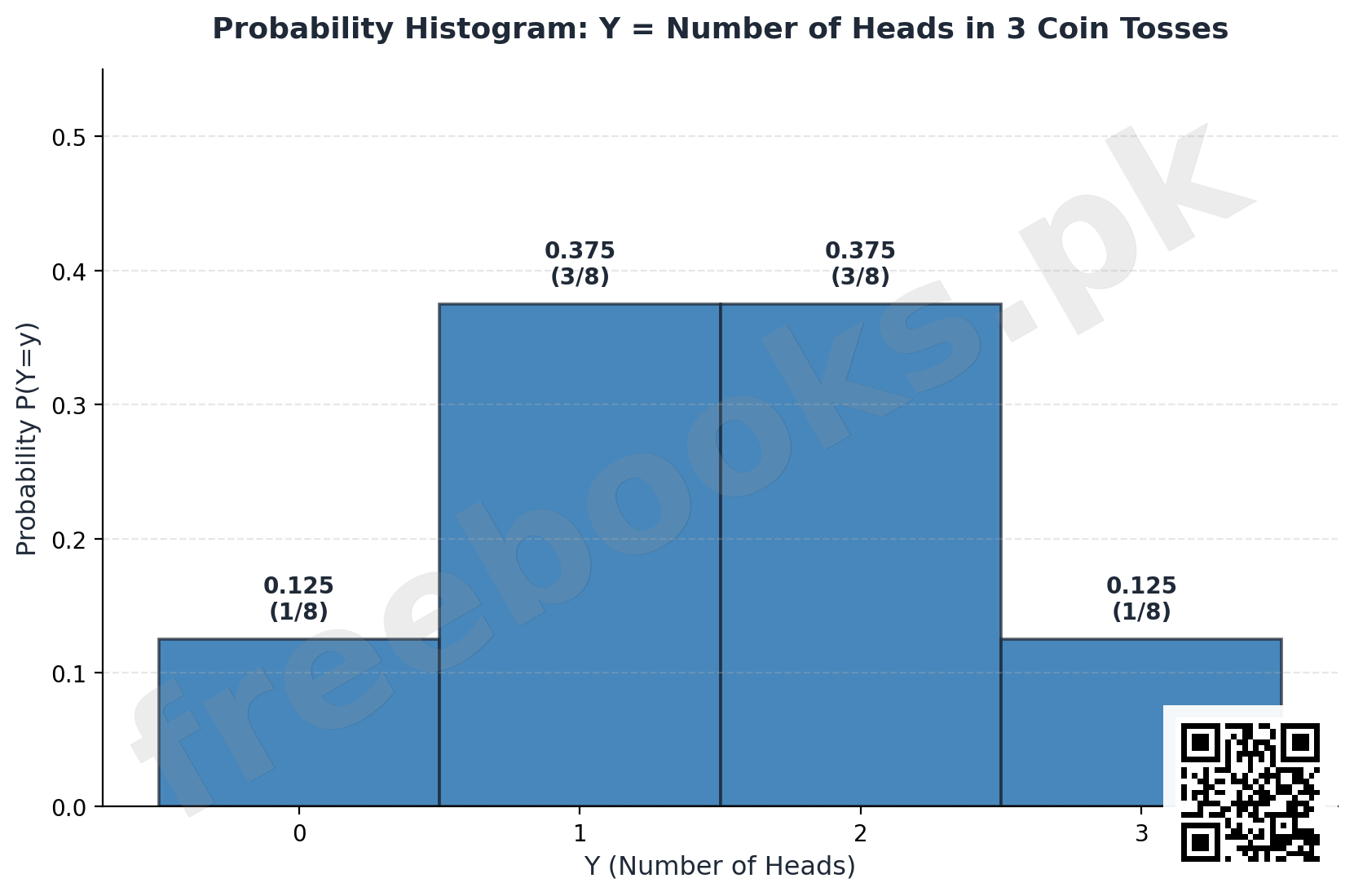
The probability mass function (PMF) of a discrete random variable Y describes the values Y can take and the probability associated with each value, usually presented in a two-column table. For example, if three coins are tossed and Y denotes the number of heads, there are 8 equally likely outcomes: no head occurs once (TTT), one head occurs 3 times (HTT, THT, TTH), two heads occurs 3 times (HHT, HTH, THH), and three heads occurs once (HHH). This gives the probability function P(Y=0)=1/8, P(Y=1)=3/8, P(Y=2)=3/8, P(Y=3)=1/8.

8.3 Probability Density Function

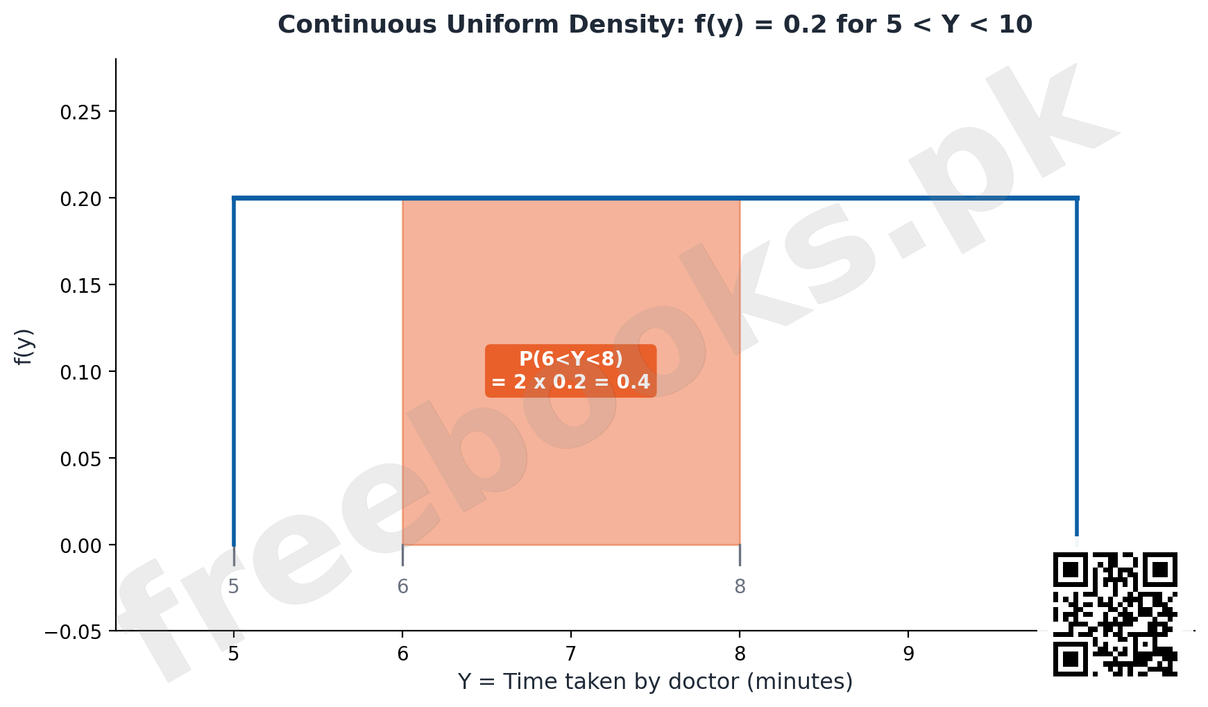
The probability density function (PDF) of a continuous random variable Y is specified by a smooth curve such that the total area under the curve equals 1. The probability that Y falls within a particular interval is the area under the curve above that interval — unlike the discrete case, we never ask for the probability at a single exact point (that probability is always zero for a continuous variable), only for probability over a range.

8.4 Discrete and Continuous Distributions, and Their Properties

A discrete uniform distribution arises when every possible value of a discrete random variable has the same probability — for example, when a fair die is thrown, each face 1 through 6 has probability 1/6, giving f(y) = 1/6 for y=1,2,…,6 and 0 otherwise. A continuous uniform distribution is defined by f(y) = 1/(b-a) for a < y < b, meaning the probability is spread evenly across the interval from a to b; when a=0 and b=1, this simplifies to f(y)=1 for 0<y<1.

For a probability mass function P(y) of a discrete random variable Y to be valid, it must satisfy two conditions: first, 0 <= P(y) <= 1 for every possible value of Y (probabilities are always between 0 and 1); second, the sum of P(y) over all possible values of Y must equal exactly 1. For a probability density function f(y) of a continuous random variable Y to be valid, it must satisfy: first, f(y) >= 0 for all y; second, the total area under the curve, P(-infinity < Y < infinity), must equal exactly 1. Not every function defined over the values of a random variable automatically qualifies as a probability distribution — both conditions must be checked and confirmed.

An important distinction: for discrete distributions, P(a <= Y <= b) is NOT equal to P(a < Y < b), because the endpoint probabilities P(Y=a) and P(Y=b) are real, nonzero quantities that must be included or excluded depending on the inequality used. For continuous distributions, however, these two probabilities ARE equal, because the probability at any single exact point is always zero (the 'area' at a single point has zero width).

8.5 Drawing the PMF and PDF

A discrete probability distribution can be drawn as a probability histogram: values of the random variable go on the x-axis, probabilities on the y-axis, and adjacent rectangles are drawn with width 1 (extending 0.5 units to each side of the value) and height equal to the probability at that point — since the width is 1, the area of each rectangle equals its probability. Alternatively, a bar chart can be drawn with thin bars (rather than full-width rectangles) whose height still equals the probability of the corresponding value. When the values of a discrete random variable become very closely spaced, the probability histogram can be approximated by a smooth curve, which is exactly the idea behind a continuous probability density function.

8.6 Expectation and Variance of a Discrete Random Variable

The mathematical expectation, or expected value, of a discrete random variable Y with probability function P(y) is defined as E(Y) = sum of y.P(y) over all values of Y. This expectation is simply the mean of the probability distribution — E(Y) is an alternative notation for the population mean, mu. Similarly, E(Y-squared) = sum of y-squared.P(y) over all values of Y.

The variance of a random variable Y is defined as sigma-squared = E[(Y – mu)-squared] = sum of (Y-mu)-squared.P(y) over all Y. Through algebraic expansion, this simplifies to the more practical computing formula: Var(Y) = E(Y-squared) – [E(Y)]-squared — exactly analogous to the shortcut variance formula used for raw data in Chapter 4.

Four key properties of expectation make calculations much easier: (i) if c is a constant, E(c) = c; (ii) if a and b are constants, E(bY plus-or-minus a) = b.E(Y) plus-or-minus a (setting a = -mu and b = 1 gives the useful result E(Y – mu) = 0); (iii) for two random variables X and Y, the expectation of their sum or difference is the sum or difference of their expectations, E(X plus-or-minus Y) = E(X) plus-or-minus E(Y); (iv) if X and Y are independent, the expectation of their product is the product of their expectations, E(XY) = E(X).E(Y).

8.9 Distribution Function (Cumulative Distribution Function)

Very often we want the probability that a random variable takes a value at or below some fixed point — for example, the chance a student scores no more than 80%, or that 5 coin tosses produce no more than 3 heads. This probability, P(Y <= y), is called the distribution function, or cumulative distribution function (CDF), and is written F(y) = P(Y <= y). For a continuous random variable, F(y) is the integral of the density function from negative infinity up to y.

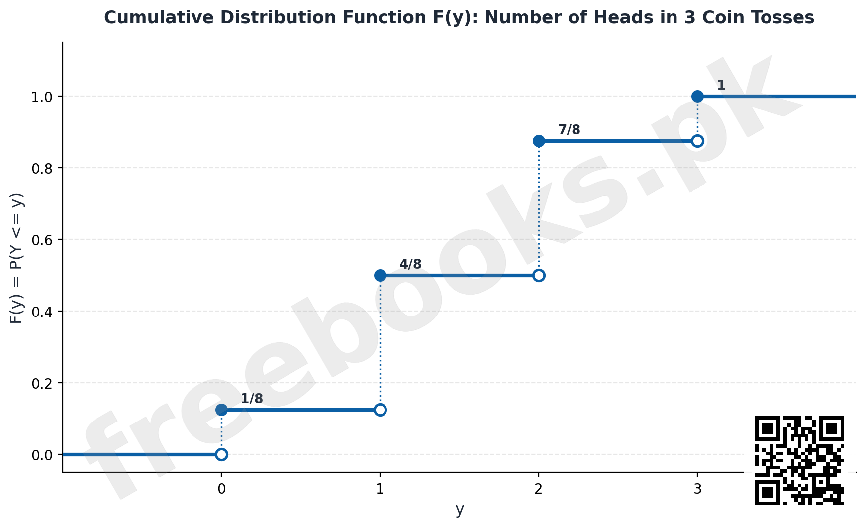
Every valid CDF satisfies four properties: (i) F(-infinity) = 0 (there's no probability of being below the smallest possible value); (ii) F(+infinity) = 1 (there's certainty of being at or below the largest possible value); (iii) F(y1) <= F(y2) whenever y1 <= y2 (the CDF is non-decreasing); (iv) F(y) is continuous at least from the right at every point. For a discrete random variable, the CDF is a step function: it jumps up by P(Y=y) at each possible value of y and stays flat (constant) in between consecutive possible values.

Important Definitions

Key Facts and Relations

Topic	Key Fact / Relation
PMF validity conditions	0 <= P(y) <= 1 for each y, and sum of P(y) over all y = 1
PDF validity conditions	f(y) >= 0 for all y, and total area under curve = 1
Discrete uniform distribution (die)	f(y) = 1/6 for y = 1,2,…,6
Continuous uniform distribution	f(y) = 1/(b-a) for a < y < b
Expected value (discrete)	E(Y) = sum y.P(y)
Variance (discrete, computing formula)	Var(Y) = E(Y^2) – [E(Y)]^2
Expectation of a constant	E(c) = c
Linear transformation of expectation	E(bY + a) = b.E(Y) + a
Expectation of sum/difference	E(X +/- Y) = E(X) +/- E(Y)
Expectation of product (independent X, Y)	E(XY) = E(X).E(Y)
Cumulative distribution function	F(y) = P(Y <= y)
Trapezoidal area rule (continuous probability)	P(a<Y<b) = [f(a)+f(b)]/2 x (b-a) (for linear density functions)

Diagrams

Probability Histogram: Number of Heads in 3 Coin Tosses: A probability histogram for the discrete random variable Y = number of heads in 3 coin tosses, with rectangles of width 1 at Y=0,1,2,3 and heights 1/8, 3/8, 3/8, 1/8 respectively, illustrating a valid probability mass function

Continuous Uniform Density: Doctor's Waiting Time: The continuous uniform density function f(y)=0.2 for 5<y<10 minutes (doctor's time with a patient), with the area between y=6 and y=8 shaded to show P(6<Y<8)=0.4, illustrating that continuous probabilities are areas under the curve

Cumulative Distribution Function: 3 Coin Tosses: The step-function cumulative distribution function F(y)=P(Y<=y) for the number of heads in 3 coin tosses, jumping from 0 to 1/8 to 4/8 to 7/8 to 1 at Y=0,1,2,3, illustrating the CDF of a discrete random variable

Short Questions & Answers

Long Questions & Answers

Explain the concept of a probability mass function and a probability density function, including the conditions each must satisfy, and explain why the treatment of probability differs between discrete and continuous random variables.

What is a probability mass function, illustrated with the three-coin example?

For a discrete random variable, the complete description of how likely each value is is called the probability mass function (PMF), pairing each possible value with its own probability, usually in a two-column table. Tossing three fair coins and letting Y represent the number of heads illustrates this: of the eight equally likely outcomes, exactly one gives zero heads, three give one head, three give two heads, and one gives three heads. Applying the classical definition of probability gives P(Y=0)=1/8, P(Y=1)=3/8, P(Y=2)=3/8, and P(Y=3)=1/8, together forming the complete PMF.

What two conditions must a valid probability mass function satisfy?

Not every function defined over a random variable's possible values automatically qualifies as a valid probability mass function; two strict conditions must hold. First, every probability the function produces must fall between 0 and 1 inclusive, since a negative probability or one exceeding 1 has no meaningful interpretation. Second, when all the probabilities across every possible value of the random variable are added together, that total must equal exactly 1, reflecting the fact that the random variable is guaranteed to take some value among all its listed possibilities.

Why does a continuous random variable need a probability density function rather than a PMF?

A continuous random variable can take infinitely many possible values within any interval, no matter how small. Because of this, it no longer makes sense to ask for the probability that the variable equals one single exact value — that probability is always mathematically zero, since a single point has zero width and therefore zero area beneath the curve above it. Instead, a probability density function (PDF) is visualized as a smooth curve over the variable's range, and probability is redefined as area: the probability the variable falls within an interval equals the area under the curve above that interval.

What two conditions must a valid probability density function satisfy?

Just as with the discrete case, an arbitrary function cannot automatically be treated as a valid probability density function without satisfying its own pair of conditions. First, the function must never dip below zero anywhere across its domain, since a negative height would imply an impossible negative area, and therefore an impossible negative probability. Second, the total area beneath the entire curve, calculated across the complete range of values the variable can take, must work out to exactly 1 — the continuous restatement of the same certainty that the variable must take some value within its full range.

Why does P(a<=Y<=b) differ from P(a<Y<b) for a discrete variable but not for a continuous one?

For a discrete random variable, P(a <= Y <= b) is genuinely different from P(a < Y < b), because the endpoint probabilities P(Y=a) and P(Y=b) are real, nonzero quantities that get included when the inequality allows 'or equal to' and excluded otherwise. For a continuous random variable, these two probabilities are always exactly equal, because the probability of landing on any single exact point is always precisely zero. Including or excluding the two endpoints therefore changes nothing about the total area being measured, and so changes nothing about the final probability.

Explain the concept of expectation (mean) and variance for a discrete random variable, state the properties of expectation, and explain the purpose and construction of the cumulative distribution function.

What is the mathematical expectation (mean) of a discrete random variable?

The mathematical expectation, or expected value, of a random variable, written E(Y), is a theoretical average calculated by taking each possible value y, multiplying it by its own probability P(y), and summing all these products across every possible value. E(Y) is nothing more than an alternative, more formal notation for the population mean, mu, that appears throughout measures of location — the difference is that here the mean is computed directly from a theoretical probability distribution rather than estimated from a finite batch of sample data.

What is the variance of a discrete random variable, and what is its computing formula?

The variance of a discrete random variable is the expected value of the squared deviation from its own mean: sigma-squared equals E[(Y – mu) squared], which unpacks to the sum, over every possible value of Y, of (Y – mu) squared multiplied by P(y). While this defining formula best shows what variance measures — the average squared spread around the centre — it is rarely the most convenient for hand computation. Algebraic simplification reduces it to the more practical computing formula Var(Y) = E(Y-squared) minus [E(Y)] squared.

What are the four key properties of expectation?

First, the expectation of any constant is that same constant: E(c) = c, since a constant never varies. Second, for constants a and b, the expectation of the linear transformation bY plus or minus a equals b times E(Y), plus or minus a — constants can be pulled outside the expectation. Third, for two random variables X and Y, the expectation of their sum or difference equals the sum or difference of their individual expectations, regardless of independence. Fourth, when X and Y are independent, E(XY) equals E(X) times E(Y), which does not hold in general when the variables are dependent.

What is the cumulative distribution function, and what shape does it take for a discrete random variable?

The cumulative distribution function (CDF), written F(y), answers questions about accumulated probability at or below a threshold, and is defined as F(y) = P(Y is less than or equal to y). For a discrete random variable, the CDF takes the distinctive shape of a step function: it stays flat across any stretch of the number line strictly between two consecutive possible values, then jumps abruptly upward by an amount equal to that value's own probability P(y) at the exact point the graph passes over each new possible value.

What four properties must every cumulative distribution function satisfy?

Every valid CDF must satisfy four properties. It must approach exactly 0 as y approaches negative infinity, since there is zero accumulated probability below the smallest possible value. It must approach exactly 1 as y approaches positive infinity, since by then every possible value has been accounted for. It must be non-decreasing throughout its domain, since accumulated probability can only increase or stay flat, never decrease. Finally, it must remain continuous at least from the right at every point, which is the technical description of its characteristic staircase-like step shape.

Multiple Choice Questions (MCQs)

Quick Revision Summary

• PMF (discrete): P(y), with 0<=P(y)<=1 for each y and sum of P(y)=1
• PDF (continuous): f(y)>=0 everywhere, total area under curve = 1; probability = area over an interval
• Discrete: P(a<=Y<=b) != P(a<Y<b). Continuous: these two ARE equal (P(Y=a)=0 always)
• Probability histogram: rectangles of width 1, height = probability, area = probability
• E(Y) = sum y.P(y) (the mean); Var(Y) = E(Y^2) – [E(Y)]^2
• Properties: E(c)=c; E(bY+a)=bE(Y)+a; E(X+/-Y)=E(X)+/-E(Y); E(XY)=E(X)E(Y) if independent
• CDF: F(y) = P(Y<=y); F(-inf)=0, F(+inf)=1, non-decreasing, step function for discrete variables

Exam Tips

• Before treating any function as a probability distribution, always check BOTH validity conditions: non-negativity and total probability/area = 1
• For continuous PDF area problems with a linear f(x), use the trapezoid formula: [f(a)+f(b)]/2 x base, rather than full integration when possible
• Remember discrete P(a<=Y<=b) includes both endpoints separately — don't confuse it with the strict-inequality version
• When computing variance, build a table with columns y, P(y), yP(y), y²P(y) to avoid arithmetic slips
• To sketch a discrete CDF, list cumulative sums of P(y) at each value, then draw a step that jumps at each value and stays flat in between