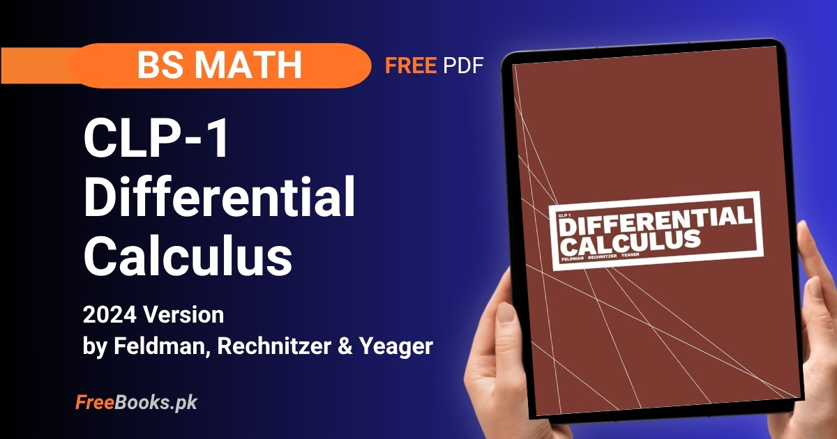
BS Mathematics and BS Engineering students can use this guide to study CLP-1 Differential Calculus by Joel Feldman, Andrew Rechnitzer and Elyse Yeager (University of British Columbia). It covers the standard Calculus I syllabus: limits and continuity, the derivative and its rules, and the applications most programmes expect — related rates, Taylor polynomials, optimisation, curve sketching and l’Hôpital’s rule — plus a short first look at antiderivatives that leads into integral calculus.
The book was written at UBC as a course text, and it reads like one: it explains why each definition looks the way it does, adds footnotes with history and side remarks, and works through around 200 numbered examples in full. Optional sections give the formal epsilon-delta definition of a limit and its proofs for students who want them, and three appendices cover high-school trigonometry, where the geometry formulas come from, and numerical root finding. One thing to know: the book is text only — it has worked examples but no end-of-section exercise sets.
Book Overview
| Course | Calculus I (differential calculus) |
| Degree Programs | BS Mathematics, BS Engineering |
| Level | University, first year — assumes high-school algebra, functions and trigonometry; Chapter 0 and Appendix A review them |
| Edition | Typeset 16 August 2024 (copyright 2016–2024); no separate edition number |
| Authors | Joel Feldman, Andrew Rechnitzer and Elyse Yeager |
| Publisher | University of British Columbia (hosted on the UBC mathematics website) |
| Structure | 5 chapters (0–4) plus 3 appendices (A–C), 426 pages |
| Exercises | None in this PDF — about 200 numbered worked examples, no end-of-section exercise sets |
| Language | English |
| License | CC BY-NC-SA 4.0 International (Creative Commons Attribution-NonCommercial-ShareAlike) |
| Format | Free PDF from the official CLP site, which also offers web-based versions of the CLP books |
Chapter List
Chapter 0: The Basics (Review)
Difficulty: Easy · Key topics: number sets N, Z, Q and R, decimal expansions, sets and interval notation, union and intersection, functions, domain and range, parse trees, inverse functions
A short memory-jogging review that the authors say will not be directly examined. It fixes names and symbols for the number systems (the natural numbers start at 1 in this book), notes that rational numbers have repeating decimals and that 0.999… is just another name for 1, then covers set notation, intervals, union and intersection. A function is defined as a rule giving exactly one output for every input in a stated set. Parse trees show how a formula is built from simple operations, an idea reused for limits and derivatives. The chapter ends with one-to-one functions, the horizontal line test and inverse functions.
Key Points:
- In this book the natural numbers
Nstart at 1;Zare the integers,Qthe rationals andRthe reals. - Rational numbers have repeating decimal expansions; irrational numbers such as
πnever repeat, and0.999... = 1because two expansions can name the same real number. - A function must be defined for every input in its domain and return exactly one output per input; it does not have to reach every element of the output set.
- Intervals:
[a, b]is closed,(a, b)is open, and the infinity end of an unbounded interval is always open. - A parse tree splits a formula into operations on numbers and
x, showing the order in which it is evaluated. - A function has an inverse only if it is one-to-one (passes the horizontal line test); the inverse’s graph is the reflection of the original in the line
y = x.
Memory Tip: Picture a function as a vending machine: every button must give something, and each button gives only one item. Two buttons may give the same item (not one-to-one), but one button never gives two items.
Common Mistake: Asking for the inverse of y = x^2 over all real numbers. It fails the horizontal line test, so the domain must first be restricted (for example to x ≥ 0) before the square root can be its inverse.
Important Questions:
- How can you tell from its graph whether a function has an inverse? Apply the horizontal line test: if every horizontal line meets the graph at most once, the function is one-to-one and has an inverse.
- Is 0.999… equal to 1? Yes. Let q = 0.999…; then 10q – q = 9, so q = 1. Both expansions are the same real number.
Chapter 1: Limits
Difficulty: Medium · Key topics: tangent lines and velocity, informal limit, one-sided limits, limit laws, 0/0 forms, squeeze theorem, limits at infinity, continuity, Intermediate Value Theorem, optional epsilon-delta definition (Sections 1.7–1.9)
Two problems motivate limits: drawing the tangent line to y = x^2 and finding the velocity of a falling ball at a single instant. The chapter gives an informal definition of a limit and shows three ways one can fail to exist: a jump between the left and right limits, wild oscillation such as sin(π/x) near 0, and growth without bound. Limit laws then handle sums, products, quotients, powers and roots. A 0/0 form is cleared by cancelling a common factor or rationalising a square root, and the squeeze theorem covers awkward cases. Limits at infinity, continuity and the Intermediate Value Theorem follow, with the formal epsilon-delta definition left to three optional sections.
Key Points:
lim(x→a) f(x) = Ldescribes whatfdoes neara; the value offataitself, or whether it is defined there, does not matter.- A two-sided limit exists only when the left-hand and right-hand limits both exist and are equal.
- The limit laws turn the limit of a sum, difference, product or quotient into the same operation on the limits, but a quotient needs the denominator’s limit to be nonzero.
- A 0/0 form is not a number; it is a hint that a common factor can be cancelled or a square root rationalised.
- Squeeze theorem: if
f ≤ g ≤ hnearaandfandhhave the same limit, thenghas that limit too. - A function is continuous at
awhen the limit exists and equalsf(a); polynomials are continuous everywhere and rational functions wherever the denominator is nonzero. - Intermediate Value Theorem: a continuous
fon[a, b]takes every value betweenf(a)andf(b)at least once.
Memory Tip: Always try plugging in first, and read the result: a number means you are done; a nonzero number over zero means the limit does not exist (or runs off to infinity); 0/0 means simplify and try again.
Common Mistake: Saying a limit does not exist just because the function is undefined at that point. (x^2 - 1)/(x - 1) is undefined at x = 1, yet its limit there is 2 once the common factor is cancelled.
Important Questions:
- In what ways can a limit fail to exist? The left and right limits can differ, the function can oscillate without settling (such as
sin(π/x)near 0), or it can grow without bound. - What does the Intermediate Value Theorem say? If
fis continuous on[a, b]andYlies betweenf(a)andf(b), thenf(c) = Yfor at least onecin[a, b]. It guarantees existence, not how many suchcthere are or where.
Chapter 2: Derivatives
Difficulty: Medium · Key topics: slope of a tangent, definition of the derivative, rates of change, product and quotient rules, the number e, derivatives of sine and cosine, chain rule, natural logarithm, implicit differentiation, inverse trig functions, Mean Value Theorem, higher derivatives (Section 2.15 optional)
Starting from the slope of a tangent to y = x^2, the chapter defines the derivative as the limit of secant slopes and reads it as an instantaneous rate of change, with the first examples worked straight from the definition. A toolbox follows: linearity, the product and quotient rules (proved in their own section), exponentials, where the number e shows up as the base whose exponential is its own derivative, and sine and cosine via a squeeze-theorem limit. The chain rule, the natural logarithm, implicit differentiation, inverse trigonometric functions, the Mean Value Theorem with Rolle’s theorem, and higher-order derivatives complete it.
Key Points:
f′(a) = lim(h→0) [f(a+h) - f(a)] / his both the slope of the tangent line atx = aand the instantaneous rate of change off.- If
fis differentiable at a point it is continuous there, but not the other way round: a corner such asy = |x|at 0 has no tangent line. - Product rule:
(fg)′ = f′g + fg′. Quotient rule:(f/g)′ = (f′g - fg′) / g^2. d/dx e^x = e^x,d/dx sin x = cos xandd/dx cos x = - sin x, with angles always measured in radians.- Chain rule:
d/dx f(g(x)) = f′(g(x)) · g′(x); it is what givesd/dx log x = 1/xonce the logarithm is treated as the inverse ofe^x. - Implicit differentiation differentiates both sides of an equation in
xandy, treatsyas a function ofx, then solves fordy/dx; it is also how the inverse trig derivatives are found. - Mean Value Theorem: if
fis continuous on[a, b]and differentiable on(a, b), somechasf′(c) = [f(b) - f(a)] / (b - a); Rolle’s theorem is the casef(a) = f(b).
Memory Tip: For the chain rule say it aloud: “derivative of the outside, evaluated at the inside, times the derivative of the inside.” For the product rule, differentiate one factor at a time and add the two results.
Common Mistake: Using the power rule on an exponential. d/dx x^2 = 2x, but d/dx 2^x is not x · 2^(x-1); the variable is in the exponent, so the exponential rule applies and brings in a factor of log 2.
Important Questions:
- What is the relationship between differentiability and continuity? A function differentiable at a point is continuous there. The converse is false, as the corner of
|x|at 0 shows. - What does the Mean Value Theorem say? Under continuity on
[a, b]and differentiability on(a, b), there is a pointcwhere the instantaneous rate of changef′(c)equals the average rate of change over the whole interval.
Chapter 3: Applications of Derivatives
Difficulty: Hard · Key topics: velocity and acceleration, related rates, exponential growth and decay, Newton’s law of cooling, Taylor polynomials and error bounds, optimisation, curve sketching, l’Hôpital’s rule
The longest chapter puts derivatives to work. Velocity and acceleration come from the first and second derivative of position, and related-rates problems link changing quantities through a geometric formula and implicit differentiation. A first look at differential equations handles carbon dating, Newton’s law of cooling and population growth by guessing exponential solutions. Section 3.4 builds Taylor polynomials from a constant to a line to a parabola to degree n and bounds the error with the next derivative. Optimisation separates local from global extrema, curve sketching gets a checklist built from f, f′ and f″, and l’Hôpital’s rule handles 0/0 and the other indeterminate forms.
Key Points:
- Velocity is
x′(t)and acceleration isx″(t); the sign of the velocity gives the direction of motion, and speed is its absolute value. - Related rates: draw and name the variables, write the equation linking them, differentiate with respect to time, and only then substitute the values at the instant asked about.
- If
dQ/dt = -kQthenQ(t) = Q(0) e^(-kt); Newton’s law of coolingdT/dt = K(T - A)givesT(t) = A + (T(0) - A) e^(Kt). - The degree-n Taylor polynomial at
ais∑ f^(k)(a) (x-a)^k / k!for k = 0 to n; the error isf^(n+1)(c) (x-a)^(n+1) / (n+1)!for somecbetweenaandx. - A global maximum or minimum on
[a, b]occurs at a critical point (f′ = 0), a singular point (f′undefined) or an endpoint; evaluatefat all of them and compare. - Sketching checklist: domain, symmetry or period, intercepts and asymptotes from
f; increasing or decreasing fromf′; concavity fromf″. - l’Hôpital: for a 0/0 or infinity/infinity form,
lim f/g = lim f′/g′provided the second limit exists; other forms are first rewritten into one of these.
Memory Tip: Read a Taylor polynomial as “match the value, then the slope, then the bend, then the next derivative, and so on” at the point a; each extra term forces one more derivative to agree.
Common Mistake: Substituting the numbers for one particular instant into a related-rates equation before differentiating. That freezes a changing quantity into a constant, so its derivative comes out as zero.
Important Questions:
- How do you find the global maximum and minimum of a continuous function on a closed interval? List every critical point, singular point and endpoint in the interval, evaluate the function at each, and take the largest and smallest values.
- When can l’Hôpital’s rule be used? When direct substitution gives 0/0 or infinity/infinity and the limit of
f′/g′exists; the limit off/gthen equals it. The hypotheses must be checked first, because the rule can fail or be circular if they are not.
Chapter 4: Towards Integral Calculus
Difficulty: Easy · Key topics: antiderivatives, the constant of integration, antiderivative of a power, 1/x and log |x|, checking by differentiation, finding the constant from extra information
A short closing section (Section 4.1, about ten pages) that gives a taste of integral calculus. An antiderivative of f is a function F whose derivative is f, and because constants differentiate to zero, every antiderivative comes with an arbitrary +c. A small table is built by reversing the derivative rules: x^n goes to x^(n+1)/(n+1) except when n = -1, where log |x| takes over, and sine, cosine and exponentials reverse in the obvious way. Answers are always checked by differentiating, extra information such as a known value pins down c, a driving problem recovers position from velocity, and the exponential-decay equation of Section 3.3 returns.
Key Points:
- An antiderivative of
fis anyFwithF′ = f; two antiderivatives of the same function differ by a constant, so the general answer is writtenF(x) + c. - Power rule in reverse: an antiderivative of
x^nisx^(n+1) / (n+1) + cforn ≠ -1. - An antiderivative of
1/xislog |x| + c, valid on any interval that does not contain 0. - Check every answer by differentiating it; a chain-rule factor (such as a 2 from
sin 2x) shows how to correct the constant in front. - A condition like
g(3) = 1together withg′fixes the value ofc.
Memory Tip: Antidifferentiation is the undo button. Differentiating a power multiplies by the exponent and lowers it by one; antidifferentiating raises the exponent by one and divides by the new exponent.
Common Mistake: Leaving out +c, or pushing x^(-1) through the power rule, which would divide by zero. The case n = -1 is the one that gives log |x|.
Important Questions:
- What is an antiderivative, and why is it not unique? It is a function whose derivative is the given function. Adding any constant leaves the derivative unchanged, so there is a whole family of antiderivatives.
- What is an antiderivative of 1/x?
log |x| + c, becaused/dx log |x| = 1/xwhereverxis not 0.
Appendices A–C: High School Material, Origin of Formulas, Root Finding
Appendix · Difficulty: Easy to Medium · Key topics: similar triangles, Pythagoras, radians, trig identities, powers and logarithms, area and volume formulas, bisection, Newton’s method, false position, secant method
Appendix A is a reference sheet of the high-school material the course assumes: similar triangles, Pythagoras, radians, trig definitions and identities, powers, logarithms, areas and volumes, ending with results you should be able to derive rather than memorise. Appendix B derives those trig, area and volume formulas, from Thales’ theorem and the sine and cosine laws to the area of a circle and the volumes of cones and spheres. Appendix C is a numerical extra on solving f(x) = 0: the bisection method, Newton’s method with an error analysis and a car-loan interest-rate example, the false position method and the secant method.
Key Points:
- Calculus uses radians throughout:
360 degrees = 2π radians, and arc length on a unit circle equals the angle. - Core identities to know cold:
sin^2 + cos^2 = 1and the double-angle formulasin 2a = 2 sin a cos a. - Bisection needs only a continuous
fwith opposite signs at the two ends; the Intermediate Value Theorem guarantees a root and each step halves the error bar. - Newton’s method steps from
x_nto the point where the tangent line crosses the x-axis,x_(n+1) = x_n - f(x_n) / f′(x_n). - The secant method replaces
f′(x_n)with the slope of a secant line through the last two guesses, so no formula for the derivative is needed. - When the starting guess is good, Newton’s method homes in on the root faster than the secant method.
Memory Tip: Bisection is safe but slow, Newton is fast but fussy about its starting guess and needs a derivative, and the secant method is Newton without the derivative.
Common Mistake: Starting Newton’s method from a bad guess. The book’s own example converges beautifully from x = 0.5 but goes astray from x = 1.5; sketch the graph first to choose a start near the root.
Important Questions:
- Why is the bisection method guaranteed to work? If
fis continuous andf(a),f(b)have opposite signs, the Intermediate Value Theorem puts a root between them; keeping the half-interval that still shows a sign change halves the error bar each step. - What is the advantage of the secant method over Newton’s method? It needs no derivative formula, since it estimates the slope from two earlier guesses, though Newton converges faster when it has a good starting point.
How to Study This Book
Read Chapters 1, 2 and 3 in order, because each one is built on the last: limits (Chapter 1) define the derivative (Chapter 2), and the derivative rules power every application in Chapter 3. Chapter 0 is a refresher the authors say will not be directly examined, so skim it and come back to Section 0.6 on inverse functions when you reach Section 2.12 on inverse trigonometric functions.
In Chapter 1 the working course is Sections 1.1–1.6. Sections 1.7, 1.8 and 1.9 are marked optional: they give the formal epsilon-delta definition of a limit, its infinite-limit version, and proofs of the limit laws. A BS Mathematics student whose course proves limits formally should read them; a student in an applied programme can safely skip them and still follow everything after.
In Chapter 2, spend your time on Sections 2.4–2.6 (the rules and plenty of examples) and Section 2.9 (the chain rule), because the rest of the book leans on them constantly. Section 2.7 includes a quick logarithm review and is where the number e appears; Section 2.10 needs the chain rule, so do not read it before Section 2.9. Section 2.5 is the proofs of the rules, and Section 2.15 is optional.
After Section 2.13 (the Mean Value Theorem), the sections of Chapter 3 are fairly independent. Sections 3.1 and 3.2 need only the chain rule and implicit differentiation, Section 3.3 needs the exponential and the natural logarithm, and Sections 3.5 and 3.6 use the consequences of the Mean Value Theorem about increasing and decreasing functions. Section 3.4 (Taylor polynomials) is the hardest in the book; read the first three approximations slowly, and treat 3.4.9, the derivation of the error formulas, as optional. Section 3.3 is only a first look at differential equations; for a full treatment pair it with Elementary Differential Equations by William Trench.
Chapter 4 is only about ten pages and works as a bridge: read it just before starting integral calculus, which the authors continue in their second book, CLP-2. Appendix A is worth a quick self-test (can you derive the results in Section A.14?), Appendix B is for readers who want to know where the formulas come from, and Appendix C fits naturally after the Intermediate Value Theorem (bisection) and after Taylor polynomials (Newton’s method).
One thing to plan for: this PDF has about 200 worked examples but no end-of-section exercise sets. The official CLP page describes the series as free textbooks and problem books, so check it for practice problems that go with this text, or practise from the exercises of another free calculus book.
What the book does not cover: integration beyond the first antiderivatives of Section 4.1, infinite series (Taylor polynomials stop at a finite degree with an error bound), hyperbolic functions, and anything with more than one variable.
Used In These Programs
This book is used for the Calculus I course in: BS Mathematics and BS Engineering programs. Browse all Differential Calculus books, all Calculus books or all Mathematics books.
Who Should Read This
CLP-1 suits a first-year BS Mathematics or BS Engineering student taking Calculus I, particularly one who wants the reasoning explained in full sentences instead of a terse definition-and-example format. It assumes high-school algebra, functions and trigonometry, with Chapter 0 and Appendix A as refreshers. It was written at the University of British Columbia and reads like a course text, and its optional sections give students heading toward analysis a first look at epsilon-delta proofs. It is not the right single choice for a student who needs a large bank of exercises, since the PDF has none, or for a course that also covers integration techniques, infinite series or several variables. A student who wants exercise sets can pair it with Calculus Volume 1 from OpenStax, which follows the same Calculus I syllabus and ends each section with practice problems.
Applicable Universities
This book is useful for students at Pakistani universities offering BS Mathematics and BS Engineering programs including Punjab University, Virtual University, COMSATS, FAST, UET, NUST, and other HEC-recognized institutions.
Official Copy of CLP-1 Differential Calculus
This book is free from its official source. Click below to open the official CLP page at the University of British Columbia, where you can download the free PDF of CLP-1 Differential Calculus.
→ Visit Official PageFAQs
Is CLP-1 Differential Calculus free?
Yes. The book’s own legal page states that it is licensed under the Creative Commons Attribution-NonCommercial-ShareAlike 4.0 International licence, with copyright held by the three authors (2016–2024). You can download it at no cost from the official CLP page, share it non-commercially with credit to the authors, and any adapted version has to carry the same licence.
Which edition is this, and is it current?
The PDF was typeset on 16 August 2024 and carries a copyright range of 2016–2024; it has no separate edition number. Differential calculus does not date the way a programming book does, so the content is current. The official page also lists a bug bounty and source files, so check it if you want to see whether a newer typesetting has been posted.
How many chapters and exercises does it have?
Five chapters (0 to 4) and three appendices (A to C) over 426 pages. It has around 200 numbered worked examples, but the PDF contains no end-of-section exercise sets. The official CLP page describes the series as free textbooks and problem books, so look there for practice problems.
Is it good for complete beginners?
It is friendly in tone and explains each idea slowly, but it assumes you already know high-school algebra, functions and trigonometry. Chapter 0 and Appendix A are quick refreshers, and the optional epsilon-delta sections can be skipped on a first read.
Does it cover integration, series or multivariable calculus?
Not beyond a first taste. Chapter 4 introduces antiderivatives in a single section, and integral calculus continues in the authors’ second book, CLP-2. The official page also lists CLP-3 Multivariable Calculus and CLP-4 Vector Calculus. Infinite series, hyperbolic functions and functions of several variables are not part of this book.
Does it cover l’Hôpital’s rule, Taylor polynomials and related rates?
Yes, all three are in Chapter 3: related rates in Section 3.2, Taylor polynomials with error bounds in Section 3.4, optimisation in Section 3.5, curve sketching in Section 3.6 and l’Hôpital’s rule with every indeterminate form in Section 3.7.
Related Books
- Calculus Volume 1 – Strang & Herman (OpenStax)
- APEX Calculus – Gregory Hartman
- Active Calculus – Matthew Boelkins
- Calculus – Gilbert Strang (MIT OpenCourseWare)
CLP-1 Differential Calculus is a free, carefully explained Calculus I text from UBC for BS Mathematics and BS Engineering students, with around 200 worked examples and optional rigorous sections. Browse more Mathematics books for the rest of your semester.
CLP-1 Differential Calculus, by Joel Feldman, Andrew Rechnitzer and Elyse Yeager, University of British Columbia. Copyright 2016–2024 the authors. Free under the Creative Commons Attribution-NonCommercial-ShareAlike 4.0 International licence. Official source: https://personal.math.ubc.ca/~CLP/
© Copyright Policy
Freebooks.pk is an educational resource for students in Pakistan. Textbooks and other books belong to their respective boards, authors and publishers, and all rights remain with them. If you are the copyright holder of any material on this page and want it changed or removed, please contact us or file a request under our DMCA policy. We review every request and remove reported content promptly.