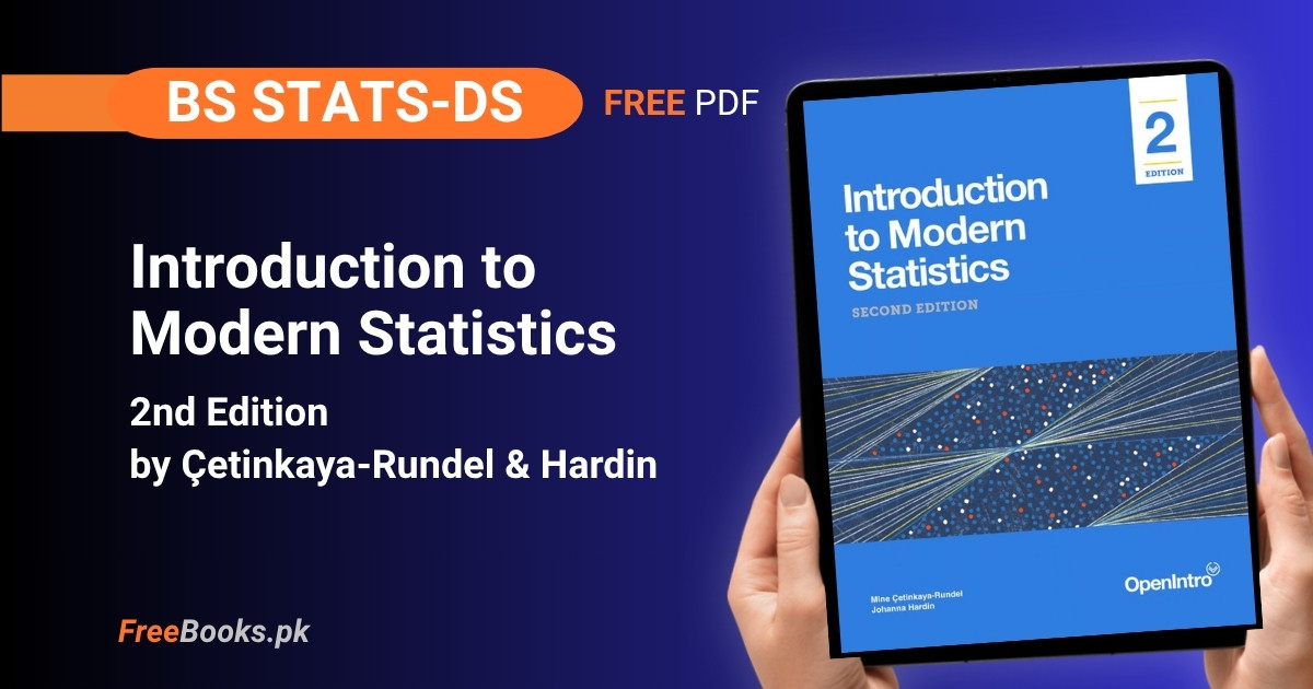
Introduction to Modern Statistics is a free, continuously-updated statistics textbook from the OpenIntro project, written by Mine Çetinkaya-Rundel and Johanna Hardin. It is part of the official syllabus material for BS Statistics and BS Data Science courses at HEC-recognized Pakistani universities, covering data collection and study design, exploratory data analysis, linear and logistic regression, and a full sequence on statistical inference built around simulation-based methods (randomization, bootstrapping) alongside the classical mathematical models.
For BS Stats/DS students, this book is built for board-style and semester exam preparation as much as for conceptual understanding: every inference chapter solves the same real dataset three different ways — by simulation, by resampling, and by formula — so a student revising for an exam can check one method’s answer against another instead of memorizing a single formula in isolation. The book’s R-based (tidyverse) worked examples double as lab material, which makes it equally useful for revision before a written exam and for a hands-on data-analysis project.
Book Overview
| Course | Modern Statistics / Introductory Statistics (R-based) |
| Degree Programs | BS Statistics, BS Data Science |
| Level | Undergraduate (introductory, no prior statistics required) |
| Author(s) | Mine Çetinkaya-Rundel & Johanna Hardin |
| Publisher | OpenIntro |
| Edition | 2nd Edition — continuously-updated free web edition |
| Structure | 6 parts · 27 chapters (23 core chapters + 4 case-study “Applications” chapters) |
| Language | English |
| License | CC BY-SA 3.0 Unported (United States) |
| Format | Free HTML (continuously updated) · PDF on Leanpub (pay-what-you-want, incl. free) |
Chapter List
Chapter 1: Hello Data
Part 1: Introduction to Data · Difficulty: Easy · Key topics: observations, variables, data frames, case study, summary tables
This chapter opens with a real randomized experiment: 451 stroke-risk patients were split into a stent-plus-medical-management treatment group (224 patients) and a medical-management-only control group (227 patients), then followed up at 30 days and 365 days. Working through the stent trial’s patient-level records and its two-way summary table teaches, before a single formula appears, what a dataset of individual cases looks like versus a summarized count table, and why the summary is usually the more useful view for a population-level question. The chapter then names the vocabulary — observations, variables, data frames — that every later chapter assumes.
Key Points:
- The stent study randomly assigned 224 patients to treatment and 227 to control, then recorded stroke outcomes at 30 and 365 days.
- An observation (case) is one unit studied; a variable is one measured characteristic of that unit.
- Raw individual-record data and a summarized count table answer the same question at different levels of detail.
- A
data framestores one case per row and one variable per column — the layout the whole book assumes.
Memory Tip: Read any new dataset the way the chapter reads the stent table — ask who the rows are before asking what the numbers mean.
Common Mistake: Trying to spot a pattern by scanning the 451-row patient table directly instead of building the 2×2 summary table first; patterns only become visible once the data is counted into groups.
Important Questions:
- In the stent study, how many patients were randomly assigned to each group? 224 patients to the treatment (stent) group and 227 to the control group.
- What is the difference between an observation and a variable? An observation is one unit being studied (one patient); a variable is one measured characteristic of that unit, such as group or 30-day outcome.
Chapter 2: Study Design
Part 1: Introduction to Data · Difficulty: Medium · Key topics: sampling strategies, experiments, observational studies, confounding, bias
This chapter asks the question every later statistical claim depends on: how were the observations actually collected? It separates sampling strategy (how units were chosen from a population) from study design (whether treatment was assigned at random), and shows why only a randomized experiment supports a causal claim while an observational study, however large, supports only an association. It works through simple random, stratified, and cluster sampling, and the biases — voluntary response, convenience sampling, non-response — that make a sample unrepresentative no matter its size.
Key Points:
- Random sampling lets a sample generalize back to its population; random assignment of treatment is what allows a causal conclusion.
- An experiment actively assigns treatment; an observational study only records what already happened.
- Voluntary response, convenience sampling, and non-response are three distinct ways a sample can be biased.
- A confounding variable is linked to both the explanatory and response variables and can create an association where no causal link exists.
- Stratified and cluster sampling are deliberate alternatives to simple random sampling, each solving a different practical constraint.
Memory Tip: Experiment = the researcher assigns treatment; Observe = the researcher only watches. Only the one that assigns can earn the word “causes.”
Common Mistake: Treating a large observational dataset as proof of causation — a bigger sample fixes precision, not the missing random assignment.
Important Questions:
- Why can a randomized experiment support a causal conclusion while an observational study cannot? Random assignment balances confounding variables across groups on average, so any outcome difference can be attributed to the treatment rather than a lurking variable.
- What is a confounding variable? A variable related to both the explanatory and response variables, capable of producing an apparent association between them even with no causal link.
Chapter 3: Applications: Data
Part 1: Introduction to Data · Difficulty: Easy · Key topics: Olympic and Paralympic 1500m data, missing categories, Simpson’s paradox
Using more than sixty years of Olympic and Paralympic 1500m gold-medal times, this case-study chapter walks through the first thing any analyst does with a brand-new dataset: inspecting its first and last rows, checking what each column represents, and noticing that in the earliest Olympiads entire categories — the Women’s division, the Paralympic visual-impairment classes T11–T13 — simply do not appear in the data. The chapter then uses the same dataset to introduce Simpson’s paradox, where a trend visible in the combined data reverses, or disappears, once a third variable such as division or era is taken into account.
Key Points:
- Inspecting both the first and last rows of a new dataset reveals different gaps or structure that a quick glance misses.
- The
paralympic_1500dataset mixes Men’s, Women’s, and T11–T13 visual-impairment classes that were not all recorded from the start. - Simpson’s paradox: an overall trend can reverse once the data is broken down by a lurking (third) variable.
- Checking for categories missing from early records is itself a data-quality step, not an afterthought.
Common Mistake: Averaging a trend across all Olympic years without checking that Women’s and Paralympic records simply did not exist for the earliest decades, silently comparing incomplete groups.
Important Questions:
- What is Simpson’s paradox? A pattern visible in aggregated data that reverses, or disappears, once the data is split by a third, lurking variable.
- Why does the 1500m dataset need a missing-category check before analysis? Because the Women’s division and several Paralympic classes were not recorded in the earliest Olympiads, so an unconditional comparison across all years would compare groups that are not actually complete.
Chapter 4: Exploring Categorical Data
Part 2: Exploratory Data Analysis · Difficulty: Easy · Key topics: contingency tables, bar plots, row/column proportions, pie charts, waffle charts
This chapter builds the full toolkit for summarizing categorical variables before any inference is attempted: contingency tables for one or two categorical variables, bar plots (including stacked, side-by-side, and standardized versions), and row versus column proportions, which answer different questions from the same table. It contrasts pie charts and waffle charts with bar plots and explains, with real multivariate examples, why a bar plot usually communicates a categorical comparison more clearly than a pie chart can.
Key Points:
- A contingency table cross-tabulates two categorical variables into counts.
- Row proportions and column proportions answer different questions from the same table — always say which one you computed.
- A segmented (standardized) bar plot shows proportions across groups even when the group sizes themselves differ.
- Pie charts make it hard for the eye to compare magnitudes; a bar plot generally communicates the same comparison more clearly.
- Waffle charts can show both the count and the proportion of a part-to-whole relationship at once.
Memory Tip: Row-vs-column proportions: the proportions always sum to 1 across whichever direction you divided by — check which way the numbers add up to confirm you computed the one you meant.
Common Mistake: Reading a row proportion as if it were a column proportion (or vice versa) — the two describe different conditional relationships and are easy to swap by accident.
Important Questions:
- What is the difference between a row proportion and a column proportion in a contingency table? A row proportion divides each cell by its row total (comparing within a row); a column proportion divides by the column total (comparing within a column) — they answer different questions.
- Why is a bar plot usually preferred over a pie chart for categorical comparisons? The human eye compares bar heights or lengths far more accurately than pie-slice angles, especially once there are more than two or three categories.
Chapter 5: Exploring Numerical Data
Part 2: Exploratory Data Analysis · Difficulty: Medium · Key topics: scatterplots, dot plots, histograms, variance, standard deviation, box plots, robust statistics, transformations
This is the chapter every later numeric-data chapter leans on. It introduces scatterplots for paired numerical data, dot plots and histograms for distribution shape, and the two standard spread measures — variance and standard deviation — alongside box plots built from quartiles and the median. It then explains robust statistics (median, IQR) as alternatives to the mean and standard deviation when a distribution is skewed or has outliers, and covers log and other transformations for taming right-skewed data before later modeling.
Key Points:
- Shape, center, and spread are the three things to describe for any numerical distribution.
- Standard deviation is the (roughly) typical distance of an observation from the mean; variance is its square.
- A box plot’s whiskers and outlier points are built from the quartiles and the 1.5×IQR rule, not from the mean and standard deviation.
- Median and IQR are robust to outliers; mean and standard deviation are not.
- A right-skewed variable (e.g., income, price) is often log-transformed before being modeled.
Practice Tip: Plot the same numerical variable as a histogram and a box plot side by side — the histogram shows shape the box plot hides, and the box plot shows outliers the histogram can bury.
Common Mistake: Reporting the mean and standard deviation for a visibly skewed variable instead of the median and IQR, which quietly overstates how “typical” the mean actually is.
Important Questions:
- When should you report the median and IQR instead of the mean and standard deviation? When the distribution is skewed or has outliers — the median and IQR are robust to extreme values while the mean and standard deviation are pulled by them.
- What rule does a box plot use to flag outliers? A point is flagged as an outlier if it falls more than 1.5 times the interquartile range (IQR) beyond the first or third quartile.
Chapter 6: Applications: Explore
Part 2: Exploratory Data Analysis · Difficulty: Easy · Key topics: effective visualization, misleading graphs, pie-to-bar comparison
This case-study chapter is about honesty in graphing, not new statistics. Using a manufacturing cost-breakdown dataset, it walks through the same data shown first as a three-dimensional pie chart and then as a plain bar plot, and shows concretely why the bar plot lets a reader’s eye compare magnitudes that the pie chart hides behind decorative color and perspective. The chapter distills this into a short set of guiding principles — keep it simple, make the scale honest, let color carry meaning — for every plot the student will build in the rest of the book.
Key Points:
- A 3-D or exploded pie chart adds visual noise without adding information.
- Color should group or distinguish categories meaningfully, not just decorate a plot.
- A bar plot generally lets a reader compare magnitudes more accurately than a pie chart, especially with more than two or three categories.
- The best plot is the one the reader can decode correctly on the first look, not the most visually elaborate one.
Memory Tip: Before publishing any chart, ask “can my reader’s eye compare the two biggest values at a glance?” — if not, simplify the chart rather than annotate it.
Important Questions:
- Why does the chapter prefer a bar plot over a pie chart for the manufacturing cost example? Because comparing bar heights is easier and more accurate for a reader than comparing pie-slice angles, particularly once there are several cost categories.
- What is the chapter’s core rule for using color in a graph? Use color only to group items or distinguish meaningful categories — not purely to make a plot look more vivid.
Chapter 7: Linear Regression with a Single Predictor
Part 3: Regression Modeling · Difficulty: Medium · Key topics: least squares, residuals, correlation, outliers, leverage
This chapter introduces simple linear regression as a way to describe — not yet test — the relationship between two numerical variables. It builds the least-squares line from residuals (the vertical distances between points and the line) and connects the slope and correlation coefficient as two views of the same linear relationship. It then separates two different kinds of unusual points: outliers in the response, and high-leverage points in the predictor, and shows that a high-leverage outlier can pull the regression line toward itself far more than an ordinary outlier can.
Key Points:
- The least-squares line minimizes the sum of squared residuals, not the sum of absolute residuals.
- Correlation (
r) measures the strength and direction of a linear relationship; it says nothing about causation. - A residual is the observed value minus the value the line predicts.
- An outlier is unusual in its response value; a high-leverage point is unusual in its predictor value.
- A high-leverage point that is also an outlier has the most influence on where the regression line ends up.
Practice Tip: After fitting any lm() model, plot the residuals against the fitted values before trusting the line — a clear pattern in that plot means a straight line is the wrong model.
Common Mistake: Quoting a strong correlation as proof that one variable causes the other — correlation measures association only, exactly as Chapter 2 warned.
Important Questions:
- What does the least-squares line actually minimize? The sum of the squared residuals (vertical distances between the observed points and the line) — not the sum of their absolute values.
- What is the difference between an outlier and a high-leverage point in regression? An outlier has an unusual response (y) value; a high-leverage point has an unusual predictor (x) value, and it is the high-leverage points that can pull the fitted line the most.
Chapter 8: Linear Regression with Multiple Predictors
Part 3: Regression Modeling · Difficulty: Medium · Key topics: indicator variables, adjusted R-squared, model selection
Building on the single-predictor model, this chapter fits a response variable against two or more predictors at once, including categorical predictors recoded as indicator (0/1) variables. It explains why plain R-squared always increases as more predictors are added — even useless ones — and introduces adjusted R-squared as a penalty for that inflation. The chapter closes with model-selection strategies for deciding which predictors earn a place in the final model rather than adding every available variable by default.
Key Points:
- A categorical predictor with k levels is represented using k−1 indicator variables plus a reference level.
- Plain R-squared can only increase (or stay the same) as more predictors are added, regardless of whether they help.
- Adjusted R-squared penalizes a model for predictors that do not meaningfully improve its fit.
- Model selection balances fit against complexity — the goal is the smallest model that still explains the response well.
Practice Tip: Compare a model’s R-squared and adjusted R-squared side by side after adding a new predictor — if adjusted R-squared drops while R-squared rises, the new variable is not pulling its weight.
Common Mistake: Adding every available variable to a multiple regression model because R-squared keeps climbing, without checking adjusted R-squared or interpretability.
Important Questions:
- Why can plain R-squared be misleading when comparing models with different numbers of predictors? Because R-squared never decreases when a predictor is added, even a predictor unrelated to the response, so it rewards complexity rather than genuine explanatory power.
- How are categorical predictors handled in a multiple regression model? They are converted into indicator (0/1) variables, using one fewer indicator than the number of categories, with one level serving as the reference.
Chapter 9: Logistic Regression
Part 3: Regression Modeling · Difficulty: Hard · Key topics: generalized linear models, log-odds, hiring-discrimination case study, unequal group sizes
This chapter extends regression to a binary (yes/no) response using logistic regression, a generalized linear model that first models the response with a binomial distribution and then models the log-odds of that distribution with a linear combination of predictors. Using a resume-callback hiring-discrimination dataset, it shows how to go from a fitted log-odds coefficient back to an interpretable odds ratio, then extends the single-predictor case to several predictors and discusses how unequal group sizes across categories complicate both estimation and interpretation.
Key Points:
- Logistic regression models the log-odds of the response, not the response probability, as a linear function of the predictors.
- A generalized linear model has two stages: a probability distribution for the response, then a linear model for that distribution’s parameter.
- Exponentiating a logistic coefficient converts it from a log-odds effect into an odds ratio.
- Odds and probability are related but are not the same number — converting between them requires the
odds = p / (1 − p)formula. - Very unequal group sizes across a categorical predictor can make its logistic coefficient unstable or hard to interpret.
Common Mistake: Interpreting a logistic regression coefficient directly as a change in probability — it is a change in log-odds, and must be exponentiated into an odds ratio before it means anything intuitive.
Important Questions:
- What does a logistic regression model actually predict? The log-odds of the binary response being a “success,” which is then transformed back into a probability or an odds ratio for interpretation.
- What are the two stages of a generalized linear model? First, choosing a probability distribution (e.g., binomial) for the response; second, modeling a parameter of that distribution with a linear combination of predictors.
Chapter 10: Applications: Model
Part 3: Regression Modeling · Difficulty: Medium · Key topics: Duke Forest housing case study, model building from raw listings
This case-study chapter takes real Duke Forest, Durham house-sale listings scraped from Zillow and walks through the full modeling workflow end to end: inspecting the raw variables (price, bed, bath, area, year built, cooling, lot size), choosing predictors, fitting a model, and checking whether the fitted price looks reasonable against the sale prices actually observed. It is deliberately a worked example rather than new theory, meant to be read right after Chapters 7–9 while those methods are still fresh.
Key Points:
- A real-estate listing dataset mixes numerical predictors (area, lot size, year built) with categorical ones (cooling type).
- The modeling workflow is: inspect variables, choose predictors, fit the model, then check the fit against reality.
- House price is a right-skewed response in most housing datasets, which is why Chapter 5’s transformation ideas resurface here.
- A model built from a single neighborhood’s sales will not automatically generalize to a different market.
Practice Tip: Before trusting the Duke Forest model’s predicted prices, sanity-check two or three of its predictions against houses you already know are over- or under-priced for their size.
Important Questions:
- What predictors does the Duke Forest case study use to model house price? Characteristics such as bedrooms, bathrooms, living area, year built, cooling type, and lot size.
- Why is house price often transformed before being modeled? Because sale prices are typically right-skewed, and a log or similar transformation makes the linear-regression assumptions a better fit.
Chapter 11: Hypothesis Testing with Randomization
Part 4: Foundations of Inference · Difficulty: Medium · Key topics: sex-discrimination case study, opportunity-cost case study, null and alternative hypotheses, p-value, randomization distribution
This is the chapter the rest of the book’s inference depends on. Using a 1970s bank-promotion sex-discrimination case and an opportunity-cost decision-making experiment as running examples, it builds the randomization (permutation) test from first principles: state a null hypothesis, repeatedly shuffle the data to simulate what the statistic would look like if the null were true, and compare the observed statistic to that simulated randomization distribution to get a p-value. Nothing here is a formula to memorize — it is a simulation procedure the student actually runs.
Key Points:
- A null hypothesis states “no effect/no difference”; the alternative states what the researcher actually suspects.
- A randomization test simulates the null hypothesis by repeatedly reshuffling group labels onto the observed data.
- The p-value is the proportion of randomized statistics at least as extreme as the one actually observed.
- A small p-value is evidence against the null hypothesis, not proof that the alternative is true.
- The sex-discrimination and opportunity-cost case studies are both revisited with the mathematical-model shortcut in Chapter 13.
Memory Tip: A randomization test answers one question: “if there really were no effect, how often would shuffled data look this extreme or more extreme by pure chance?” — the p-value is just that proportion.
Common Mistake: Saying a p-value is “the probability the null hypothesis is true” — it is the probability of data this extreme (or more) given that the null hypothesis is true, which is a different statement.
Important Questions:
- How does a randomization test simulate the null hypothesis? By repeatedly reshuffling the observed group labels (or data) and recalculating the statistic each time, generating a distribution of what the statistic would look like if there were truly no effect.
- What does the p-value actually measure? The proportion of the randomization distribution that is at least as extreme as the observed statistic, assuming the null hypothesis is true.
Chapter 12: Confidence Intervals with Bootstrapping
Part 4: Foundations of Inference · Difficulty: Medium · Key topics: medical-consultant case study, tappers-and-listeners case study, bootstrap resampling, confidence interval
Where Chapter 11 asked “is there an effect?”, this chapter asks “how big is it, with how much uncertainty?” It introduces bootstrapping — resampling with replacement from the one sample already in hand, rather than from the whole population — as a practical stand-in for the impossible-in-practice step of collecting many fresh samples. Two case studies, a medical-consultant decision scenario and a musical tappers-and-listeners experiment, are used to build bootstrap distributions and read a confidence interval directly off the middle of that resampled distribution.
Key Points:
- Bootstrapping resamples with replacement from the original sample to approximate sample-to-sample variability.
- A confidence interval is a range of plausible values for the population parameter, built from the spread of the bootstrap distribution.
- A wider bootstrap distribution means more uncertainty in the original estimate; a narrower one means less.
- Bootstrapping does not require assuming the null hypothesis is true — it estimates variability around whatever the sample actually showed.
Memory Tip: Randomization shuffles to test “no effect”; bootstrapping resamples to measure “how much does my estimate wobble?” — different question, different simulation.
Common Mistake: Interpreting a 95% confidence interval as “there is a 95% chance the true parameter is in this interval” — the correct reading is about the long-run success rate of the method across repeated samples, not a probability statement about this one interval.
Important Questions:
- What is the key difference between bootstrapping and the randomization test from Chapter 11? Bootstrapping resamples with replacement from the observed sample to estimate variability of an estimate; a randomization test reshuffles the data to simulate the null hypothesis being true.
- How is a confidence interval read off a bootstrap distribution? By taking the middle portion of the bootstrap distribution that matches the desired confidence level (e.g., the middle 95% for a 95% interval).
Chapter 13: Inference with Mathematical Models
Part 4: Foundations of Inference · Difficulty: Hard · Key topics: Central Limit Theorem, normal distribution, standard error, opportunity-cost and stent case studies revisited
This chapter re-solves the same opportunity-cost, medical-consultant, and stent problems from Chapters 11–12, but this time with a mathematical shortcut instead of a simulation: the Central Limit Theorem, which says that for a large enough sample, a sample proportion or sample mean’s own distribution across repeated samples is approximately normal. Once that approximation holds, a standard error formula replaces the thousands of simulated resamples, producing the same p-values and confidence intervals as the computational methods — which is the chapter’s central point: the three methods are different roads to the same destination.
Key Points:
- The Central Limit Theorem says a sample statistic’s distribution across repeated samples approaches a normal shape as sample size grows.
- The standard error is the standard deviation of a statistic’s sampling distribution, estimated from one sample.
- A normal-model-based p-value or confidence interval should closely match the randomization or bootstrap version for the same data, when sample size is large enough.
- Mathematical models require checking technical conditions (e.g., sample size, independence) that randomization and bootstrapping do not need as strictly.
Memory Tip: Think of Chapters 11–13 as three cameras pointed at the same scene — randomization, bootstrapping, and the normal-model shortcut should all show roughly the same picture when the sample is large enough.
Common Mistake: Reaching for the normal-model formula without first checking its sample-size and independence conditions — the shortcut only works when those conditions actually hold.
Important Questions:
- What does the Central Limit Theorem allow a statistician to do? It justifies approximating the sampling distribution of a statistic (like a sample mean or proportion) with a normal distribution once the sample size is large enough, enabling formula-based inference.
- Why should a mathematical-model result be checked against a randomization or bootstrap result for the same data? Because the mathematical model depends on technical conditions holding; comparing it against the computational methods is a sanity check that those conditions were reasonable.
Chapter 14: Decision Errors
Part 4: Foundations of Inference · Difficulty: Medium · Key topics: Type I and Type II error, significance level, two-sided tests, power
Every hypothesis test from Chapter 11 onward can be wrong in two different ways, and this chapter names and quantifies both: a Type I error (rejecting a true null hypothesis) and a Type II error (failing to reject a false one). It formalizes the significance level (α) as the Type I error rate a researcher is willing to accept, contrasts one-sided and two-sided hypotheses, and introduces statistical power — the probability of correctly detecting a real effect — as the quantity that governs how large a study’s sample size needs to be.
Key Points:
- A Type I error rejects a true null hypothesis (a “false positive”); a Type II error fails to reject a false null hypothesis (a “false negative”).
- The significance level, α, is the Type I error rate the researcher chooses before seeing the data, commonly 0.05.
- A two-sided hypothesis test splits the significance level across both tails of the distribution; a one-sided test puts it all in one tail.
- Power is the probability of correctly rejecting a false null hypothesis — it increases with larger sample size and larger true effect size.
- Lowering the Type I error rate (stricter α) generally raises the Type II error rate, for a fixed sample size.
Memory Tip: Type I is “crying wolf” when there is none; Type II is staying silent when the wolf is real.
Common Mistake: Treating α = 0.05 as a universal, context-free rule rather than a choice that should depend on the real-world cost of a false positive versus a false negative.
Important Questions:
- What is the difference between a Type I and a Type II error? A Type I error rejects a true null hypothesis; a Type II error fails to reject a false null hypothesis.
- What happens to power as sample size increases? Power increases, because a larger sample makes it easier to detect a real effect of a given size.
Chapter 15: Applications: Foundations
Part 4: Foundations of Inference · Difficulty: Medium · Key topics: method comparison recap, malaria-vaccine case study
This chapter is the hinge of the whole book: a recap table that lines up randomization, bootstrapping, and mathematical models side by side against the same set of questions (what varies, what the method assumes, when it applies), followed by a malaria-vaccine clinical-trial case study worked through using more than one of the three methods so the student sees them converge on the same real-world conclusion rather than as three unrelated procedures from three unrelated chapters.
Key Points:
- Randomization, bootstrapping, and mathematical models are three different ways to quantify the same underlying sampling variability.
- Randomization simulates the null hypothesis; bootstrapping estimates variability around an observed estimate; mathematical models rely on a theoretical approximation (usually the Central Limit Theorem).
- The malaria-vaccine case study is deliberately solved more than one way to show the methods agree when their conditions hold.
- Choosing a method is a question of which technical conditions are met and which question (testing vs. estimating) is being asked, not personal preference.
Memory Tip: Keep the Chapter 15 recap table open while reading Parts 5 and 6 — every new inference chapter from here on is just this table applied to a new data situation.
Important Questions:
- What is the purpose of the Part 4 recap table? To summarize, side by side, how randomization, bootstrapping, and mathematical models each handle the same inferential questions, so the three methods are seen as related rather than separate topics.
- Why is the malaria-vaccine case study solved with more than one inference method? To demonstrate that the methods converge on the same real-world conclusion when their respective conditions are satisfied.
Chapter 16: Inference for a Single Proportion
Part 5: Statistical Inference · Difficulty: Medium · Key topics: bootstrap test for a proportion, normal approximation, success-failure condition
This chapter applies the three Part 4 methods to the simplest categorical data structure: one binary variable summarized as a single sample proportion. It builds both a bootstrap-based test and confidence interval for a proportion and the mathematical-model (normal-approximation) version, and introduces the success-failure condition — at least 10 expected successes and 10 expected failures — as the technical check that decides whether the normal-model shortcut is trustworthy for a given sample.
Key Points:
- A sample proportion summarizes one binary variable across all observations.
- The success-failure condition requires at least 10 expected successes and 10 expected failures for the normal approximation to apply.
- When the success-failure condition fails, the bootstrap or randomization approach from Part 4 is the more trustworthy option.
- The standard error of a sample proportion depends on both the proportion itself and the sample size.
Practice Tip: Before running a normal-model test or interval for a proportion, check the success-failure condition first — if it fails, fall back to the bootstrap methods from Chapter 12 instead of forcing the formula.
Common Mistake: Applying the normal-approximation formula to a proportion test with a very small or very large sample proportion without checking that at least 10 successes and 10 failures are expected.
Important Questions:
- What is the success-failure condition, and why does it matter? It requires at least 10 expected successes and 10 expected failures in the sample; without it, the normal approximation used for a proportion’s mathematical model is not reliable.
- What should be done if the success-failure condition fails for a proportion test? Use the bootstrap or randomization-based methods instead, since they do not depend on the normal approximation holding.
Chapter 17: Inference for Comparing Two Proportions
Part 5: Statistical Inference · Difficulty: Medium · Key topics: difference in proportions, randomization test, bootstrap interval, pooled standard error
This chapter extends Chapter 16 to two independent groups, building a point estimate for the difference in proportions (p̂₁ − p̂₂) and then testing and estimating that difference with all three Part 4 methods in turn: a randomization test that permutes group labels, a bootstrap confidence interval, and a normal-model test that uses a pooled standard error under the null hypothesis of no difference.
Key Points:
- The natural point estimate for comparing two groups’ proportions is the difference
p̂₁ −p̂₂. - A randomization test for two proportions permutes the group labels while holding the outcomes fixed.
- Under the null hypothesis of no difference, the standard error calculation pools the two groups’ data together.
- The success-failure condition must be checked separately within each of the two groups, not just on the combined sample.
Common Mistake: Using the unpooled standard error formula (appropriate for a confidence interval) when testing the null hypothesis of no difference, where the pooled formula is the correct one.
Important Questions:
- What is the point estimate used when comparing two independent proportions? The difference between the two sample proportions,
p̂₁ −p̂₂. - Why does the hypothesis test for two proportions use a pooled standard error while the confidence interval does not? Because the null hypothesis assumes the two population proportions are equal, so the test pools the data to estimate that one common proportion; the confidence interval makes no such assumption.
Chapter 18: Inference for Two-Way Tables
Part 5: Statistical Inference · Difficulty: Medium · Key topics: chi-square test of independence, two-way tables, expected counts
Once either variable in a comparison has more than two levels, a simple difference of proportions is no longer well defined, and this chapter introduces the chi-square test of independence for exactly that situation. It builds the test statistic from the squared difference between observed and expected counts in a two-way table, explains why bootstrapping does not apply here (there is no single population parameter to resample toward), and works through both the randomization version and the mathematical chi-square approximation.
Key Points:
- A two-way table with more than two levels in either variable has no single proportion to summarize the relationship, unlike Chapters 16–17.
- The chi-square statistic sums the squared, standardized differences between observed and expected counts across every cell.
- Expected counts under independence are computed from the table’s row and column totals.
- Bootstrapping is not used for two-way tables because there is no single population parameter whose variability it would estimate.
Memory Tip: Chi-square asks one question across every cell at once: “how far are the observed counts from what independence would predict?”
Important Questions:
- Why can’t bootstrapping be used for a two-way table test of independence? Because there is no single population parameter being estimated; the test is about independence between two categorical variables, not about estimating one value’s variability.
- How is an expected count calculated for a cell in a two-way table under the independence assumption? By multiplying that cell’s row total by its column total and dividing by the overall table total.
Chapter 19: Inference for a Single Mean
Part 5: Statistical Inference · Difficulty: Medium · Key topics: bootstrap interval for a mean, t-distribution, degrees of freedom
Moving from categorical to numerical data, this chapter builds inference for a single numeric response variable’s mean: a bootstrap confidence interval, and the mathematical-model version that, unlike the proportion chapters, uses the t-distribution rather than the normal distribution because the population standard deviation is unknown and must itself be estimated from the sample. It introduces degrees of freedom as the quantity that controls how much heavier the t-distribution’s tails are compared with the normal distribution for a small sample.
Key Points:
- Inference for a single mean uses the t-distribution, not the normal distribution, because the population standard deviation is estimated rather than known.
- Degrees of freedom for a one-sample t-procedure equal the sample size minus one.
- As sample size (and degrees of freedom) grows, the t-distribution approaches the normal distribution.
- A t-distribution has heavier tails than the normal distribution, which widens confidence intervals for small samples.
Practice Tip: For a small sample, compare the t-interval to what a normal-based interval would have given — the t-interval should be visibly wider, which is the heavier tails doing their job.
Common Mistake: Using the normal distribution instead of the t-distribution for a small-sample mean, which understates the true uncertainty in the estimate.
Important Questions:
- Why does inference for a single mean use the t-distribution rather than the normal distribution? Because the population standard deviation is unknown and must be estimated from the sample, which adds extra uncertainty that the t-distribution’s heavier tails account for.
- How are degrees of freedom calculated for a one-sample t-procedure? Degrees of freedom equal the sample size minus one.
Chapter 20: Inference for Comparing Two Independent Means
Part 5: Statistical Inference · Difficulty: Medium · Key topics: difference in means, randomization test, Welch’s t-test
This chapter extends Chapter 19 to two independent groups, forming the point estimate x̄₁ − x̄₂ and testing or estimating it with a randomization test, a bootstrap interval, and a t-based mathematical model whose standard error combines the variability of both groups. It carefully separates the hypothesis-test formula, which assumes no difference between the groups, from the confidence-interval formula, which estimates the size of a difference that may or may not be zero.
Key Points:
- The point estimate for comparing two independent means is
x̄₁ −x̄₂. - The standard error for a difference in two independent means combines the standard errors of both groups, not just one.
- Degrees of freedom for the two-sample t-procedure are typically approximated rather than a simple sum of each group’s degrees of freedom.
- A randomization test for two means permutes group labels across the combined data to simulate “no difference.”
Common Mistake: Assuming the two groups must have equal variances before using a two-sample t-test — the standard (Welch-style) approach in this chapter does not require that assumption.
Important Questions:
- What point estimate is used when comparing two independent sample means? The difference between the two sample means,
x̄₁ −x̄₂. - How does a randomization test simulate “no difference” between two independent groups? By pooling all observations together and repeatedly reassigning them at random to the two group labels, then recomputing the difference in means each time.
Chapter 21: Inference for Comparing Paired Means
Part 5: Statistical Inference · Difficulty: Medium · Key topics: paired data, dependence, mean paired difference
This chapter handles the case Chapter 20’s independence assumption rules out: two measurements that are linked, such as before-and-after readings on the same subject. It shows that pairing collapses two numeric variables into one new variable — the paired difference — which converts the problem back into the single-mean inference already covered in Chapter 19, now applied via a randomization test, a bootstrap interval, and the mathematical (t-based) model for the mean paired difference.
Key Points:
- Paired data means each observation in one group is linked to a specific observation in the other group (e.g., the same subject measured twice).
- Pairing converts two dependent numeric variables into one new variable: the difference within each pair.
- Once reduced to differences, the single-mean methods from Chapter 19 apply directly.
- Treating paired data as if it were two independent samples ignores the dependence and typically understates precision.
Memory Tip: If you can draw a line connecting each “before” point to its own “after” point, the data is paired — take the differences first, then treat them as one single-mean problem.
Common Mistake: Running a two-independent-means test (Chapter 20) on data that is actually paired, which ignores the dependence between the two measurements and gives a misleading standard error.
Important Questions:
- How does pairing simplify the analysis of two dependent numeric variables? By converting the pair of measurements into a single new variable, the within-pair difference, which can then be analyzed with single-mean methods.
- What mistake occurs if paired data is analyzed as if the two groups were independent? The dependence between the paired measurements is ignored, which usually produces an incorrect (often inflated) standard error and misleading conclusions.
Chapter 22: Inference for Comparing Many Means
Part 5: Statistical Inference · Difficulty: Hard · Key topics: baseball batting-average case study, ANOVA, F-statistic, randomization test for many groups
This chapter moves beyond two groups to three or more, using a baseball batting-average case study to motivate why a simple pairwise difference no longer captures the comparison once there are several groups to consider at once. It introduces Analysis of Variance (ANOVA) and its F-statistic, which compares variability between group means to variability within groups, and builds both a randomization version and the mathematical F-distribution version of the same test.
Key Points:
- ANOVA tests whether three or more group means are all equal, rather than comparing them two at a time.
- The F-statistic compares the variability between group means to the variability within groups.
- A large F-statistic suggests the group means differ more than within-group noise alone would explain.
- ANOVA’s overall test does not by itself say which specific groups differ — that requires a follow-up comparison.
Memory Tip: ANOVA’s whole idea in one phrase: “is the spread between the group averages bigger than the spread inside each group?”
Common Mistake: Running repeated two-sample t-tests on every pair of groups instead of a single ANOVA, which inflates the overall false-positive rate across all the comparisons.
Important Questions:
- What does the F-statistic in ANOVA actually compare? The variability between the group means to the variability within each group.
- Why is running many separate two-sample t-tests a worse approach than ANOVA when comparing three or more groups? Because performing multiple pairwise tests inflates the overall chance of at least one false positive, while ANOVA tests all the group means together in a single, properly calibrated test.
Chapter 23: Applications: Infer
Part 5: Statistical Inference · Difficulty: Medium · Key topics: method recap, redundant-adjectives linguistics case study
This chapter closes Part 5 with two recap tables — one for the computational methods (randomization, bootstrapping) and one for the mathematical models (normal, t, chi-square, F) — and a linguistics case study on the order of redundant adjectives (why “big red barn” sounds right but “red big barn” does not) that applies the chapter’s inference toolkit to a question with no obvious “right” numeric answer in advance, which is exactly the point of practicing it here.
Key Points:
- Part 5 covered inference for one and two proportions, two-way tables, one and two means, paired means, and many means — eight data structures in total.
- Each data structure, where appropriate, was analyzed using all three Part 4 methods: randomization, bootstrapping, and a mathematical model.
- The redundant-adjectives case study shows the same toolkit applied to a genuinely open linguistic research question, not a textbook-manufactured one.
- Recognizing which of the eight data structures a new problem matches is the actual skill Part 5 is building, more than any single formula.
Important Questions:
- How many distinct data structures does Part 5 cover inference methods for? Eight: single proportion, two proportions, two-way tables, single mean, two independent means, paired means, many means (ANOVA), and the recap itself.
- What is the point of the redundant-adjectives case study at the end of Part 5? To show the inference toolkit applied to a real, open-ended linguistics question rather than a manufactured textbook example.
Chapter 24: Inference for Linear Regression with a Single Predictor
Part 6: Inferential Modeling · Difficulty: Hard · Key topics: sandwich-store case study, slope inference, randomization test for slope, bootstrap for slope, checking model conditions
This chapter returns to the single-predictor regression line from Chapter 7 and asks whether its slope is real or could plausibly be zero. Using a sandwich-store sales case study, it builds a randomization test for the slope, a bootstrap confidence interval for the slope, and the mathematical t-test and interval version, then spends real time on checking the technical conditions — linearity, constant variance, normal residuals, independence — that decide whether the mathematical shortcut can be trusted for a given dataset.
Key Points:
- Testing a regression slope against zero asks whether the predictor has any linear relationship with the response at all.
- A randomization test for the slope permutes one variable relative to the other to simulate “no relationship.”
- The mathematical t-test for a slope requires checking linearity, constant variance, nearly normal residuals, and independent observations.
- A statistically significant slope is not automatically a practically important one — effect size still matters.
Common Mistake: Reporting a regression slope’s p-value without first checking the residual plots for linearity and constant variance — a wrong-shaped model can still produce a small p-value.
Important Questions:
- What null hypothesis is tested when checking whether a regression slope is “significant”? That the true population slope is zero — i.e., no linear relationship between the predictor and the response.
- What four technical conditions should be checked before trusting the mathematical model for a regression slope? Linearity, constant variance of residuals, nearly normal residuals, and independence of observations.
Chapter 25: Inference for Linear Regression with Multiple Predictors
Part 6: Inferential Modeling · Difficulty: Hard · Key topics: regression software output, multicollinearity, cross-validation, prediction error
This chapter reads a full multiple-regression software printout line by line — coefficients, standard errors, t-statistics, p-values — and asks what each individually tests for. It then tackles multicollinearity, where two or more predictors carry overlapping information and inflate each other’s standard errors, making individual coefficients unstable even when the overall model fits well. The chapter closes with cross-validation as an honest, out-of-sample way to assess how well the model will actually predict new data rather than just how well it fits the data it was built on.
Key Points:
- Each coefficient’s individual p-value tests whether that one predictor is useful given all the other predictors already in the model.
- Multicollinearity inflates standard errors and can make an individually important predictor’s coefficient look statistically insignificant.
- A model can fit its training data well and still predict new data poorly — the two are different questions.
- Cross-validation splits data into folds to estimate out-of-sample prediction error rather than relying on in-sample fit statistics alone.
Practice Tip: Before trusting an individual coefficient’s p-value in a multiple regression, check the predictors for correlation with each other — high multicollinearity is often the real explanation for a “surprising” result.
Common Mistake: Dropping a predictor from a model purely because its own p-value looks large, without checking whether multicollinearity with another predictor is the actual cause.
Important Questions:
- What problem does multicollinearity cause in a multiple regression model? It inflates the standard errors of the correlated predictors’ coefficients, which can make individually useful predictors appear statistically insignificant.
- Why is cross-validation used alongside in-sample fit statistics? Because a model can fit the data it was trained on well while still predicting new, unseen data poorly; cross-validation estimates that out-of-sample performance directly.
Chapter 26: Inference for Logistic Regression
Part 6: Inferential Modeling · Difficulty: Hard · Key topics: model diagnostics, software output for logistic models, cross-validation for classification
This chapter closes the book’s main sequence by combining Chapter 9’s logistic regression with the inferential ideas from Parts 4 and 6: reading a logistic model’s software output for coefficient significance, running diagnostic checks appropriate to a binary response rather than a numeric one, and using cross-validation — now adapted to a classification setting — to assess how well the fitted model will classify genuinely new cases rather than the ones it was trained on.
Key Points:
- Diagnostics for a logistic model differ from a linear model’s residual plots because the response is binary, not continuous.
- A logistic model’s software output reports coefficients on the log-odds scale, which must be exponentiated to read as odds ratios.
- Cross-validation for a classification model evaluates prediction accuracy (or a related metric) on held-out cases, not model fit on the training data.
- The inferential ideas here build directly on Chapter 9’s descriptive logistic model and Chapter 25’s cross-validation approach.
Common Mistake: Judging a logistic model’s quality purely by how well it classifies the data it was trained on, rather than its cross-validated performance on new cases.
Important Questions:
- Why can’t the same residual diagnostics used for linear regression be applied directly to logistic regression? Because the response variable in logistic regression is binary rather than continuous, so diagnostics appropriate to that structure are needed instead.
- What does cross-validation evaluate for a logistic regression model? How accurately the model classifies cases it was not trained on, which is a better measure of real-world performance than training-data fit alone.
Chapter 27: Applications: Model and Infer
Part 6: Inferential Modeling · Difficulty: Hard · Key topics: Mario Kart eBay-auction case study, multiple regression with inference, controlling for variables
The book’s closing chapter applies the full Part 6 toolkit to 141 real eBay auctions of the Mario Kart video game, modeling total auction price against characteristics like auction duration, item condition, and the number of Wii-wheel accessories included, while holding the other characteristics constant. It is the book’s final demonstration that a single multiple regression model, read correctly with its inferential output, can answer several distinct practical questions (“does a longer auction raise or lower price, controlling for everything else?”) from one fitted model.
Key Points:
- The
mariokartdataset records 141 eBay auctions with variables including price, condition, duration, and accessory count. - “Controlling for” other variables means interpreting one coefficient’s effect while the rest of the model’s predictors are held fixed.
- Indicator variables (e.g., new vs. used condition) are interpreted the same way here as in Chapter 8’s descriptive model.
- A single well-specified multiple regression model can answer several different practical questions at once, each read from a different coefficient.
Important Questions:
- What does “controlling for other variables” mean when interpreting a coefficient in the Mario Kart model? It means reading that one predictor’s effect on price while holding every other predictor in the model fixed.
- What practical questions does the Mario Kart case study use multiple regression to answer? Questions such as whether longer auctions are associated with higher or lower prices, and how much buyers pay on average for extra Wii-wheel accessories, each while controlling for the auction’s other characteristics.
Download Introduction to Modern Statistics (Free)
Click below to open the official OpenIntro page for this book — it links straight to the free, continuously-updated web edition and the pay-what-you-want (including free) Leanpub PDF.
↓ Download PDFHow to Study This Book
Read Part 1 (Chapters 1–3) first no matter your background. It is short, but it sets the vocabulary — observations, variables, sampling versus random assignment, Simpson’s paradox — that every later chapter assumes without re-explaining.
Spend real time in Part 2 (Chapters 4–6) before moving on. The book deliberately slows down here: every plot type introduced — bar plots, histograms, box plots, scatterplots — is reused without re-introduction in every chapter from Part 3 onward, so rushing past Part 2 makes later chapters harder, not easier.
Part 3 (Chapters 7–10) covers regression as description only — no hypothesis testing yet. A student who only needs descriptive modeling for a research-methods or data-analysis course, rather than a full statistics sequence, can treat Chapters 7, 8, and 10 as a self-contained unit and treat Chapter 9 (logistic regression) as optional unless the course needs a binary outcome.
Part 4 (Chapters 11–15) is the hinge of the entire book. Read it in order: Chapter 11 (randomization), Chapter 12 (bootstrapping), Chapter 13 (the mathematical shortcut), Chapter 14 (the errors both still carry), Chapter 15 (the recap). Skipping straight to Part 5 without these five chapters turns every later inference chapter into a list of unrelated formulas instead of three repeated applications of one idea.
Part 5 (Chapters 16–23) applies the Part 4 toolkit to one new data structure per chapter — one proportion, two proportions, a two-way table, one mean, two means, paired means, many means (ANOVA), then a recap. A one-semester introductory course typically assigns four or five of these eight chapters rather than all of them; check your syllabus before assuming you need every one.
Part 6 (Chapters 24–27) combines modeling (Part 3) with inference (Part 4), and genuinely requires both as prerequisites — this is not a part to read out of order. It is usually the last three to four weeks of a two-semester introductory sequence, or the entire content of a dedicated regression-and-modeling course.
What the book never covers: Bayesian inference, time series, multi-factor ANOVA, and any probability theory beyond what Chapter 13’s Central Limit Theorem needs. A BS Statistics or BS Data Science student planning further theory should pair this book with a calculus-based mathematics text for the limit and series machinery this book’s Chapter 13 uses but does not derive.
Each core chapter’s “Interactive R tutorials” and “R labs” pointers (and the four standalone Applications chapters, which are built around them) assume RStudio access, since the book is written around the tidyverse, infer, and openintro R packages. A reader without R can still read every chapter’s prose, Key Points, and case studies in full; only the hands-on lab exercises require the software.
Used In These Programs
This book is used for the Modern Statistics / Introductory Statistics course in: BS Statistics · BS Data Science. Browse all Statistics-tagged books or the full Statistics category on Freebooks.pk.
Who Should Read This
Introduction to Modern Statistics is written for a first or second college statistics course aimed at BS Statistics and BS Data Science majors who want a rigorous introduction that leans on simulation — randomization and bootstrapping — before it leans on formulas, and only brings in the normal and t-distributions once the student has already seen what those models are approximating. It assumes no prior statistics course and only the R basics the book itself teaches through the openintro and tidyverse packages, so it is not the right starting point for a student who already wants a measure-theoretic, formula-first treatment of probability and distributions — for that deeper mathematical foundation, pair it with a book like Calculus Volume 1, which builds the limit and integral machinery that Chapter 13’s Central Limit Theorem leans on without deriving. It is also not the right fit for a student who wants a pure R-programming reference; here, the code is always in service of the statistics, not the other way around.
Applicable Universities
This book is useful for students at Pakistani universities offering BS Statistics, BS Data Science, and related BS Mathematics or Computer Science degrees, including Punjab University, Virtual University, COMSATS, FAST, UET, NUST, and other HEC-recognized institutions.
FAQs
Is Introduction to Modern Statistics free?
Yes. The full text is free to read online at the book’s official OpenIntro page under a CC BY-SA 3.0 Unported (United States) license, and the PDF on Leanpub is pay-what-you-want, including $0.
Which edition is this?
This is the 2nd Edition, which is a continuously-updated free web book rather than a single fixed print date. The older 1st Edition (openintro-ims1.netlify.app) is still online for courses that have not switched over yet.
How many chapters does it have?
27 chapters across 6 parts — 23 core content chapters plus 4 case-study “Applications” chapters, one near the end of most parts — along with end-of-chapter exercises and R labs/tutorials for every part.
Is it good for complete beginners?
Yes for statistics itself — it assumes no prior statistics course and builds every idea from first principles using real case studies. It assumes only the R basics the book teaches as it goes, so a student with zero R experience should expect the early R labs to take extra time.
Does it cover simulation-based methods, or just classical formulas?
Both, deliberately side by side: every major inference chapter is solved with a randomization test, a bootstrap interval, and the classical mathematical (normal/t/chi-square/F) model, so students see all three approaches converge on the same answer rather than learning only one.
Do I need to already know R programming to use this book?
No. The book is built around the openintro, tidyverse, and infer R packages and the prose explains the statistics regardless of R background, but every chapter’s labs and interactive tutorials assume RStudio access, so a short R primer alongside Chapters 1–2 is recommended for a student with no coding background at all.
Related Books
- Calculus Volume 1 PDF Download – Strang & Herman (OpenStax)
- Discrete Mathematics: An Open Introduction PDF Download – Oscar Levin (4th Edition)
- Active Calculus PDF Download – Matthew Boelkins (2nd Edition)
Introduction to Modern Statistics takes a BS Statistics or BS Data Science student from the first definition of a variable all the way to inferential regression modeling, using real case studies — stent trials, hiring discrimination, eBay auctions — instead of invented numbers, and showing the simulation and formula-based methods side by side at every step. Browse more Statistics books on Freebooks.pk.
Introduction to Modern Statistics, 2nd Edition, by Mine Çetinkaya-Rundel and Johanna Hardin. Published by OpenIntro under a Creative Commons Attribution-ShareAlike 3.0 Unported (United States) License. Official source: openintro.org/book/ims.
© Copyright Policy
Freebooks.pk is an educational resource for students in Pakistan. Textbooks and other books belong to their respective boards, authors and publishers, and all rights remain with them. If you are the copyright holder of any material on this page and want it changed or removed, please contact us or file a request under our DMCA policy. We review every request and remove reported content promptly.